How To Make Google Sheets Not Round

Google Sheets is a powerful tool that many individuals and businesses use to manage their data and perform calculations. However, one frustrating feature of Sheets is its tendency to automatically round numbers. This can be especially problematic for those who need to maintain precise values, such as financial analysts or scientists.

Fortunately, there is a way to prevent Google Sheets from rounding your numbers. In this tutorial, we will explore the different methods you can use to keep your numbers from being rounded, and maintain their accuracy and precision. Before we dive into the specifics of how to prevent Google Sheets from rounding numbers, it’s important to understand why Sheets rounds numbers in the first place. Sheets rounds numbers by default to make them easier to read and understand. This can be helpful for certain applications, but in some cases, it can lead to incorrect calculations or analysis. With that in mind, let’s explore some methods for keeping your numbers precise in Google Sheets.

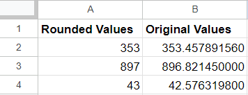
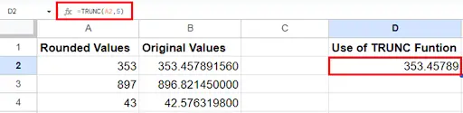
Suppose we have the following values (shown in column B) that have been rounded by Google Sheets (column A) by default. To keep them in decimal places, you can use the following methods.

Method 1 – Use Increase Decimal Places Option

The Increase Decimal Places option in the Google Sheets toolbar allows you to increase the number of decimal places displayed for a number in a cell. This is useful if you want to see a more precise value for a number that has many decimal places.

Step 1 – Select Cell

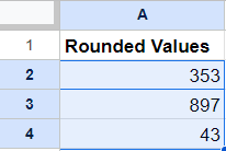
• Click on the cell or range of cells that contains the number you want to adjust.

Step 2 – Click On The “Increase Decimal Places” Button In The Toolbar

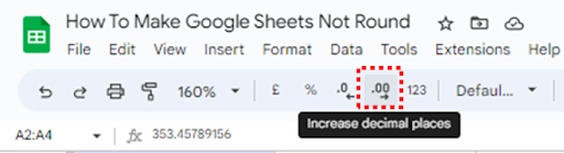
• In the Google Sheets Toolbar, click on the “Increase Decimal Places” button. This button looks like a set of numbers with an upward-pointing arrow to the right.

Step 3 – Increase The Decimal Places As Needed

• Click on the “Increase Decimal Places” button repeatedly to increase the number of decimal places displayed in the cell. Each time you click the button, the number of decimal places will increase by one.
• Stop increasing the number of decimal places when you have the desired level of precision for the number. Be aware that increasing the number of decimal places beyond what is necessary can make the number more difficult to read.

That’s it! You have successfully used the “Increasing Decimal Places” option in the Google Sheets Toolbar.

Method 2 – Use Of TRUNC Function

The TRUNC function in Google Sheets is used to truncate a number to a specified number of decimal places or to remove the decimal portion of a number altogether. This function can be useful if you need to work with whole numbers or if you want to round a number down to a specific level of precision.

Syntax of TRUNC Function

=TRUNC(Value, [places])

• Value: the number to be truncated.
• Places: [Optional] The number of significant digits to the right of the decimal point to retain.

To use the TRUNC function in Google Sheets, follow these steps:

Step 1 – Select the cell where you want to use the TRUNC function

• Click on the cell where you want to apply the TRUNC function.

Step 2 – Type The TRUNC Function

• In the selected cell, type the following formula:
• =TRUNC(value, [place]).
• For our example, we will truncate the numbers up to five decimal places, the formula would be =TRUNC(A2, 5). Note that the place argument is optional, and if you don’t include it, the function will truncate the number to zero decimal places by default.
• Press enter to display the result.

Step 3 – Drag The Formula To Apply It To Other Cell

• If you want to apply the TRUNC function to other cells, you can simply drag the formula to apply it to those cells.
• That’s it! You have successfully used the TRUNC function in Google Sheets.