How to make data table in Google Sheets
In this tutorial, we will show you how you can use formulas and other features in Google Sheets to build some desirable features that will make your tables less error-prone and more effective at conveying information. The major steps are given below;
Google Sheets is a web-based spreadsheet application provided by Google, offering similar functionality to Excel but with the advantage of collaborative editing and cloud storage. Creating tables in Google Sheets is essential for organizing, analyzing, and visualizing data effectively. It promotes collaboration, simplifies data management, and provides powerful tools for data manipulation and exploration, making it an invaluable resource for individuals and teams working with data.
Step 1 – Create a spreadsheet and name the columns

– To create a new sheet click on the “+” button or select “Blank” to create a new blank sheet.
– In the first row, enter the column headers for your data. Each column header should represent a different attribute or variable.
– In the subsequent rows, enter your data values under each column.
Step 2 – Convert the data into a table
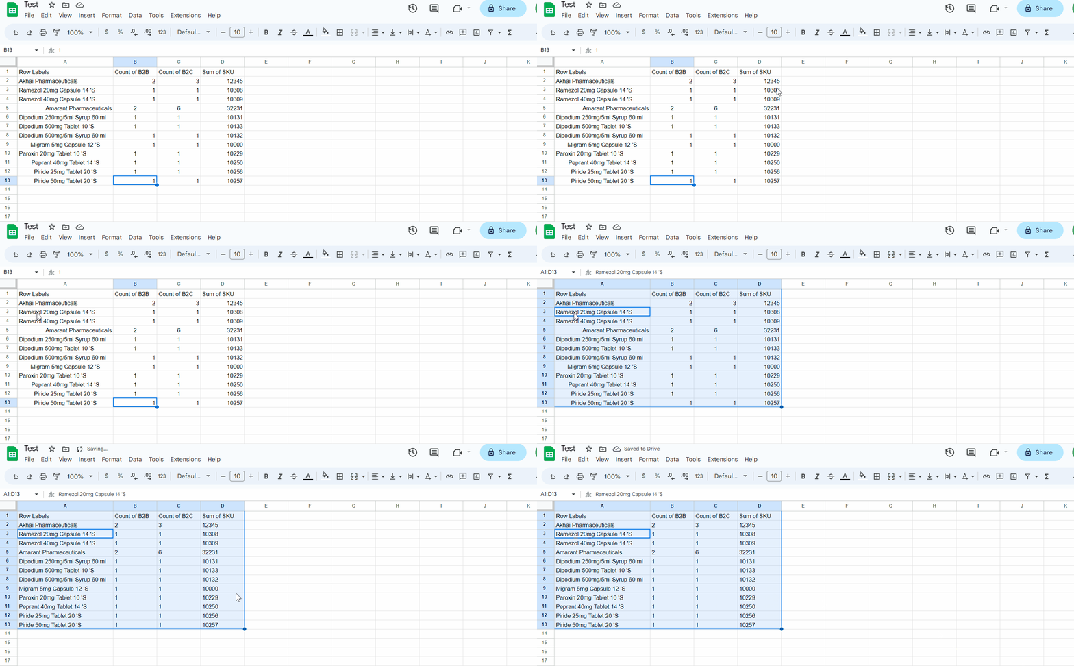
– To convert the data into a table in Google Sheets press the keyboard shortcut key.
– Select the range of cells containing your data, including the column headers. Then, go to the “Format” menu and choose “Table” from the dropdown. Alternatively, you can press Ctrl+Shift+L (Windows) or Command+Shift+L (Mac) to apply the table format.
– All the data will be aligned left
Step 3 – Customize the table
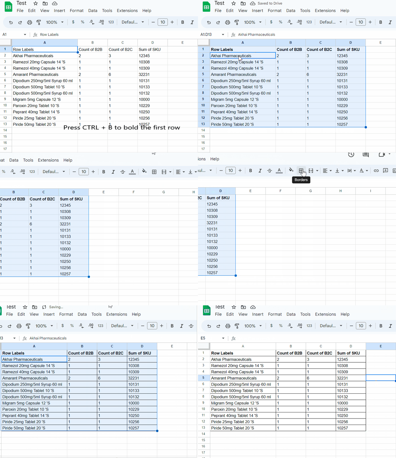
– Make the header bold by selecting the data and pressing the B button on the icon bar or press the keyboard shortcut CTRL + B.
– Select all the data and apply the borders by clicking on the border button in the icon bar.
– Click on the first option All Borders.
Step 4 – Sum the formula in a column
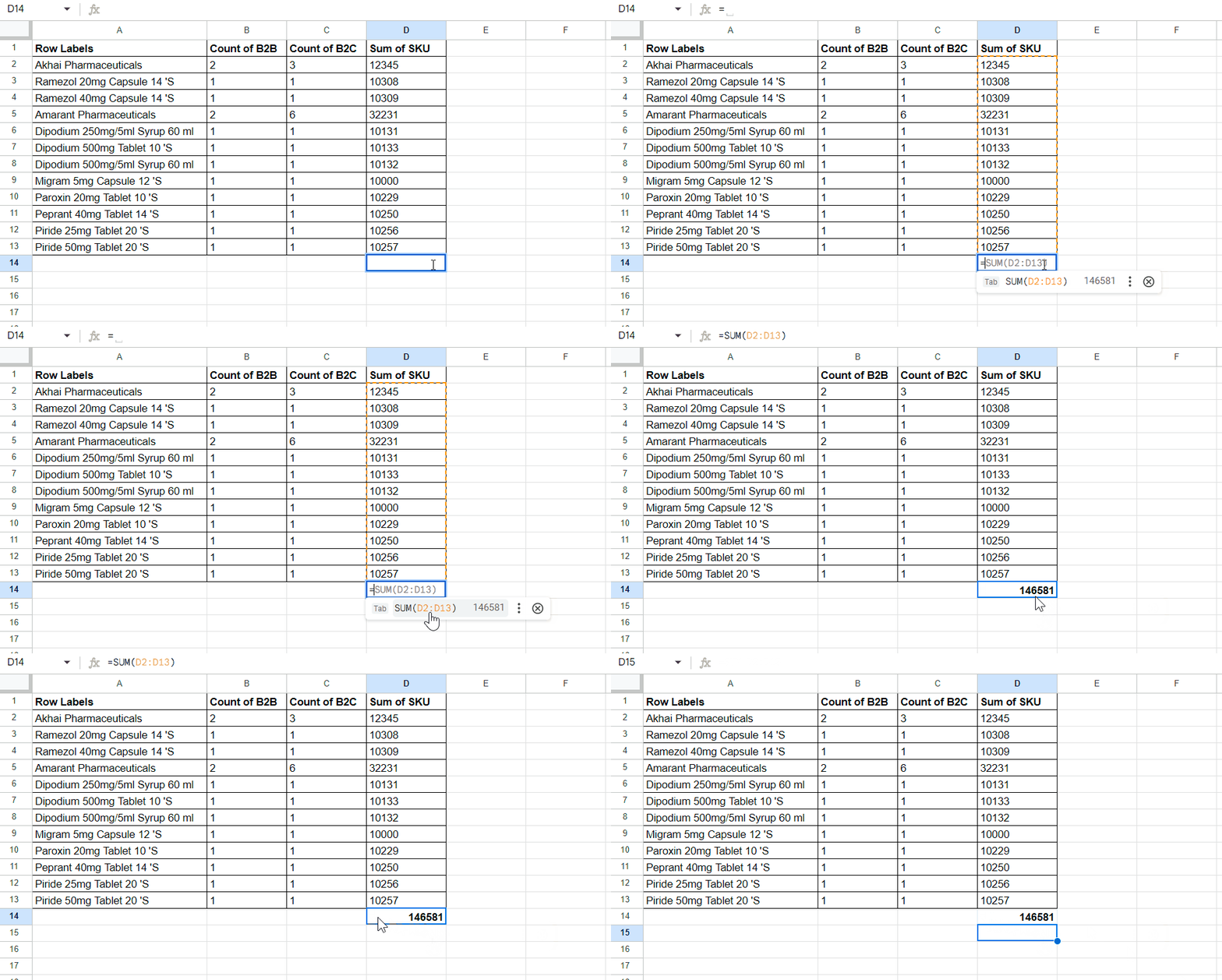
– To make the table data-oriented, we would add different formulae in different columns. In this case, we apply a SUM formula in column D.
– In this case, we apply the formula as =SUM(D2:D13).
– As soon as you press the enter key, it will add the whole column’s numeric values as total in cell D14
Step 5 – Apply an Average formula
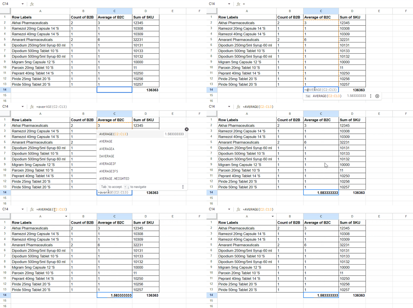
– To apply the average formula, In this case, we apply an Average formula in column C.
– In this case, we apply the formula as =AVERAGE(C2:C13).
– As soon as you press the enter key, it will make an average of the entire column’s numeric values as total in cell C14
Step 6 – Apply the count formula

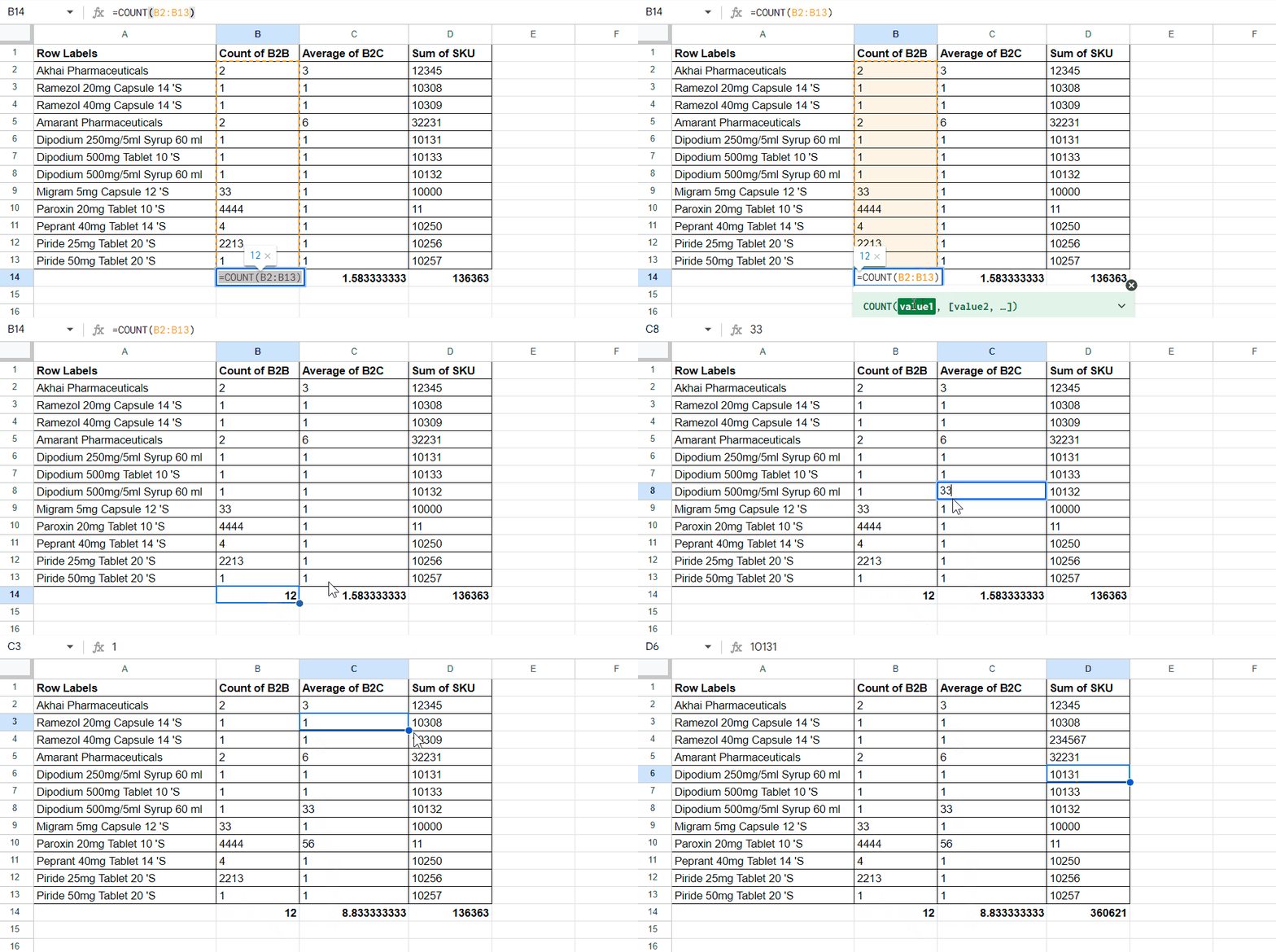
– To apply the count formula, In this case, we apply a Count formula in column B to count the total number of rows/entries.
– In this case, we apply the formula as =COUNT(B2:B13)
– As soon as you press the enter key, it will make an average of entire column’s numeric values as a total in cell B14


