
How to make a comparison table in Excel
 By
SpreadCheaters
By
SpreadCheaters
In this tutorial, we will learn how to make comparison tables in Excel using Conditional formatting. Suppose we have a dataset containing the attendance records of students for a week. Each day, two attendance records are taken for each student. Our objective is to create a comparison table to analyze and compare the attendance of each student.
Microsoft Excel enables the creation of comparison tables with seemingly random data. By analyzing and comparing this data, valuable insights are gained, aiding in important real-life decision-making, particularly in business contexts.
Step 1 – First Select Second Table
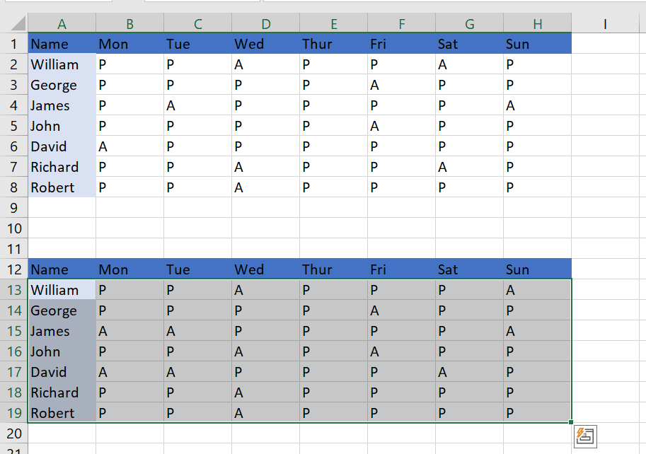
– Firstly select the second Table in the datasheet.
Step 2 – Locate the Conditional Formatting Menu in the Home Tab
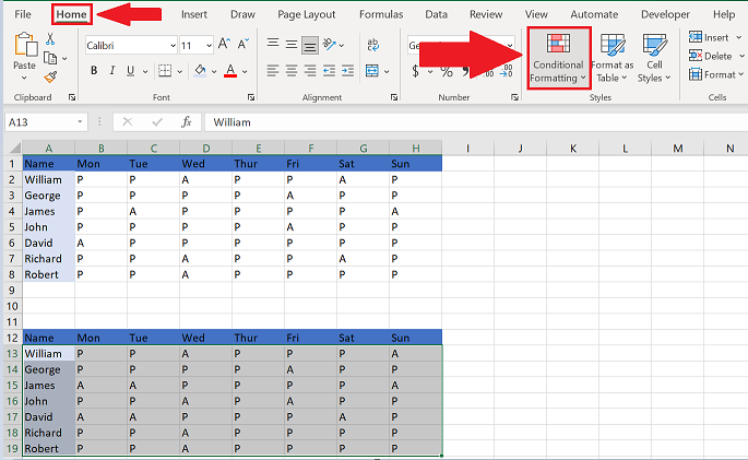
– Now from the list of the main menu, on the home tab locate conditional formatting in the styles group.
Step 3 – Select the New Rule Option
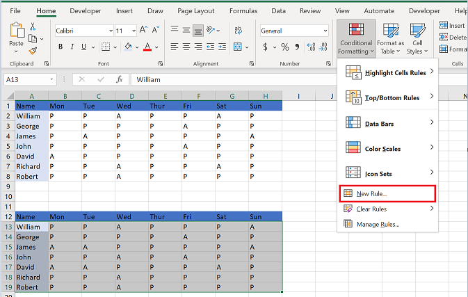
– Select the new rule option in the drop-down menu.
Step 4 – Select the Rule Type
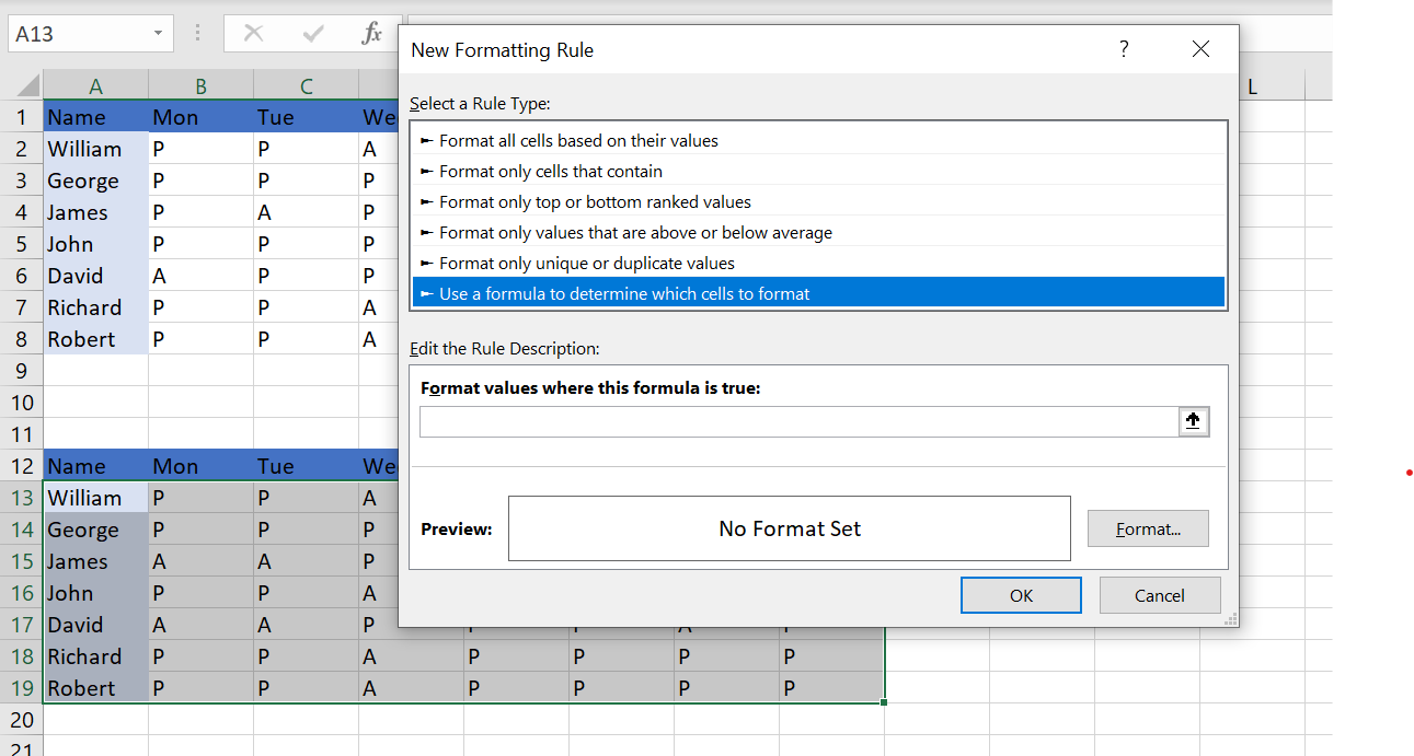
– Select the “Use a formula to determine which cells to format” in the rule type from the new dialog box.
Step 5 – Enter the Formula
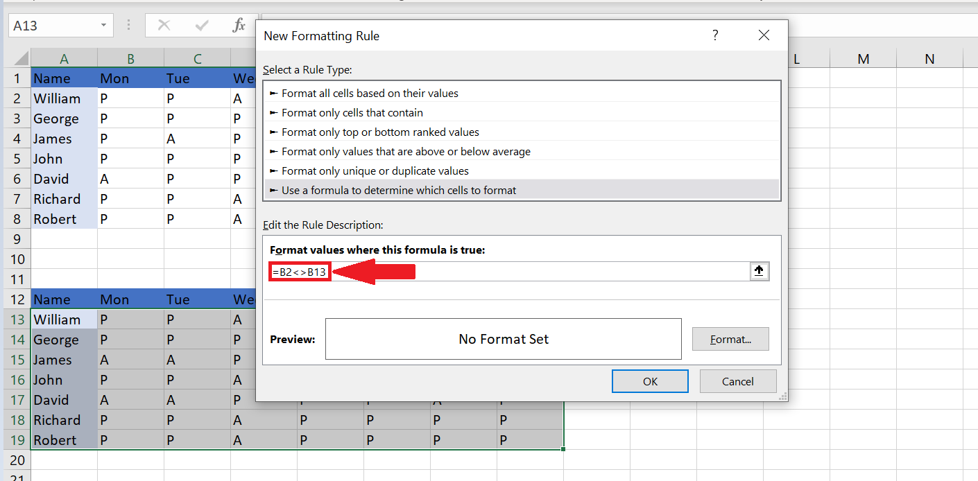
– Enter the following formula in the field “Format values where this formula is true”.
=B2<>B13.
Step 6 – Click the format button
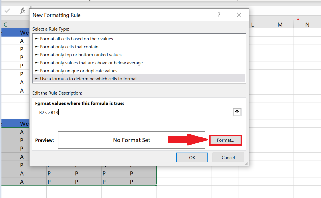
– After that click the format button
Step 7 – Locate the Fill Tab And Choose Color
– Select the fill tab and choose a color of your choice and press “Ok”.
Step 8 – Hit “Ok”
– Again hit ok to make a comparison table.


