
How to do conditional formatting based on another column in Excel
 By
SpreadCheaters
By
SpreadCheaters
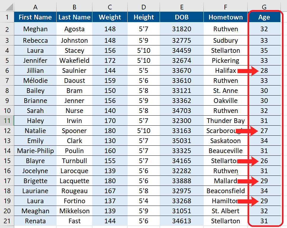
Let’s look at this data set which consists of the details about the hockey team players. We wish to highlight those players whose ages are less than 30 years. We’ll achieve this by using conditional formatting and following the steps explained in the forthcoming sections.
Conditional formatting is an amazing feature of Excel which helps us to highlight desired data based on some conditions. In this tutorial we’ll learn how we can use this feature to highlight a data range based upon the values in another column.
Step 1 – Select the data range to highlight through conditional formatting
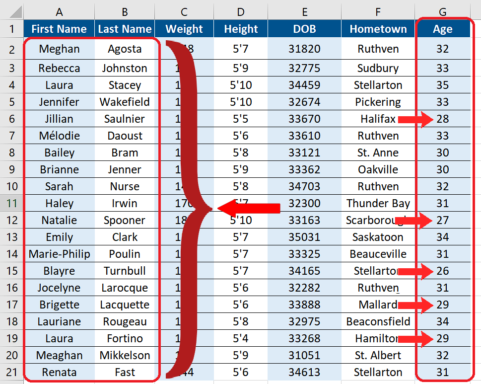
– Select the data range which we want to highlight. In our case the data range A2:B21 will consist first and last names of the players as shown above.
Step 2 – Go to Home tab
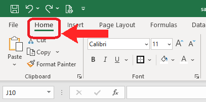
– Now go to the Home tab.
Step 3 – Go to Styles group
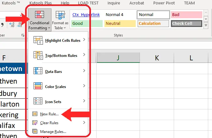
– Now go to the Styles group -> Conditional Formatting -> New Rule.
Step 4 – Write the formula to do conditional formatting
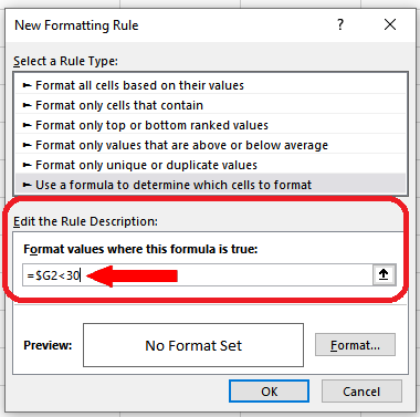
– Write the following formula in the conditional formatting formula bar;
= $G2 < 30
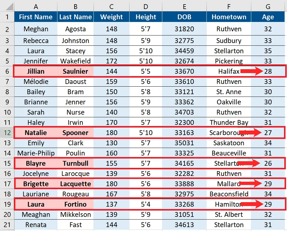
The above formula tells Excel to highlight all the cells in row 2 of selected data range i.e. A2:B21, only if the value in the cell G2 is less than 30. The same process will be repeated for all the rows of the data range i.e. from row 2 to row 21. The trick here is the use of dollar sign ($) before the column name $G. This locks the column name to be checked for applying the conditional formatting on A2:B21.
Step 5 – Set the format for conditional formatting
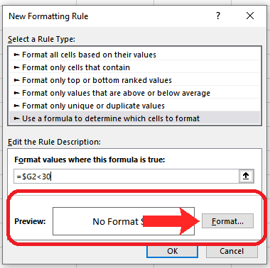
– Click on the format tab so that we can choose formatting styles to highlight our data range.
Step 6 – Set the font to bold for conditional formatting
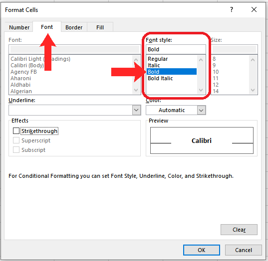
– In the next dialog box, click on the Font tab and select Bold.
Step 7 – Set the suitable colour for conditional formatting
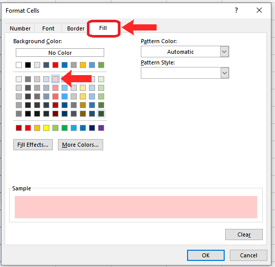
– In the same dialog box, click on the Fill tab and select an appropriate colour for highlighting the data.
Step 8 – Click on Apply to use conditional formatting
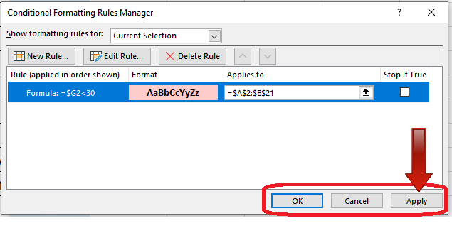
– When you click on the OK button in the last step, you will see the following window.
Step 9 – Implement the conditional formatting rules
– Click on OK again. This will implement the conditional formatting rules to the selected data range.


