How to lock cells in Google Sheets

Locking cells in Google Sheets refers to the process of preventing the content of a cell from being edited, moved, or deleted. This is particularly useful when working with sensitive or critical data, such as financial information or complex formulas. By locking specific cells or ranges of cells, you can ensure that they remain unchanged and secure, while still allowing other users to interact with other parts of the spreadsheet.

In this tutorial, we will learn how to lock cells in Google Sheets. To lock cells in Google Sheets, you can use the “Protect sheets and ranges” feature. This can be accessed from the “Data” menu and allows you to select specific cells or ranges that you want to protect. You can then choose to restrict users from editing, to comment, or even viewing the protected cells. We have a spreadsheet that contains three columns: Names, Total Marks, and Obtained Marks. Our goal is to prevent any changes to the Names and Total Marks columns by locking them.

Method 1: Using the Data Tab to Lock Cells

In this method, we’ll use the options which are available under the Data tab present on the list of main tabs in Google Sheets.

Step 1 – Go to the Data Tab 

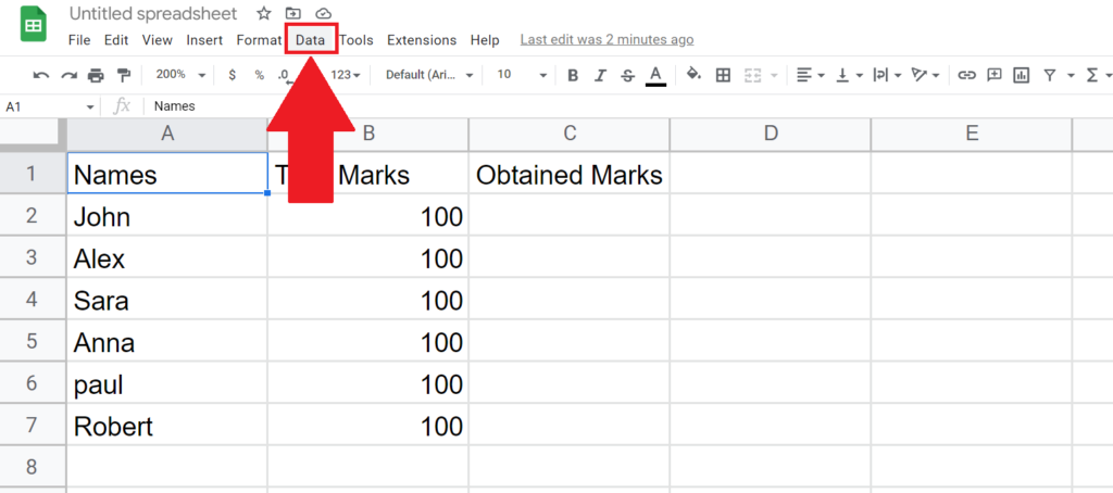
• Go to the Data tab in the menu bar.
• A drop-down menu will appear.

Step 2 – Click on the Protect Sheets and Ranges

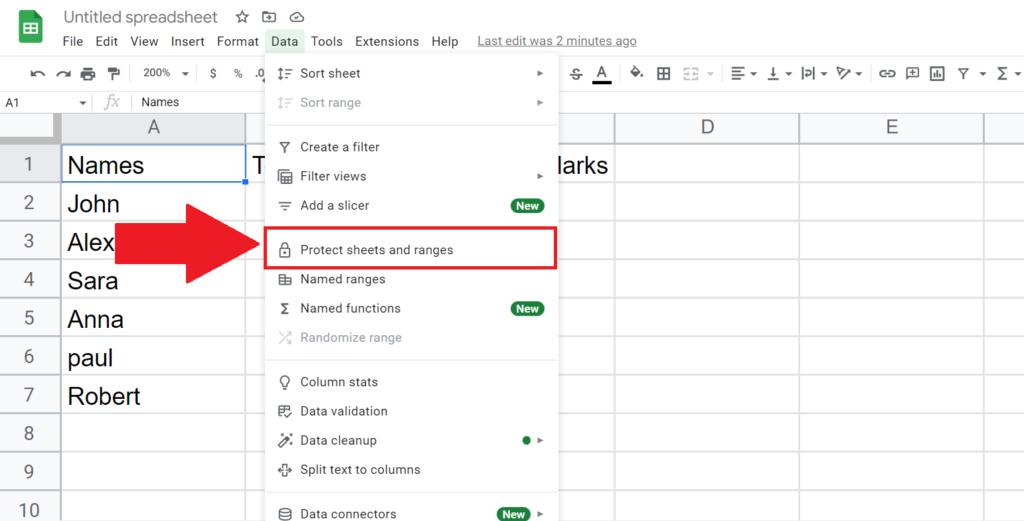
• Click on the Protect Sheets and Ranges option in the drop-down menu.

Step 3 – Click on “Add a sheet or Range” 

• Click on the “Add a Sheet or range” option.

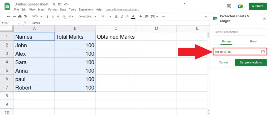
Step 4 – Enter the Range of the Cells 

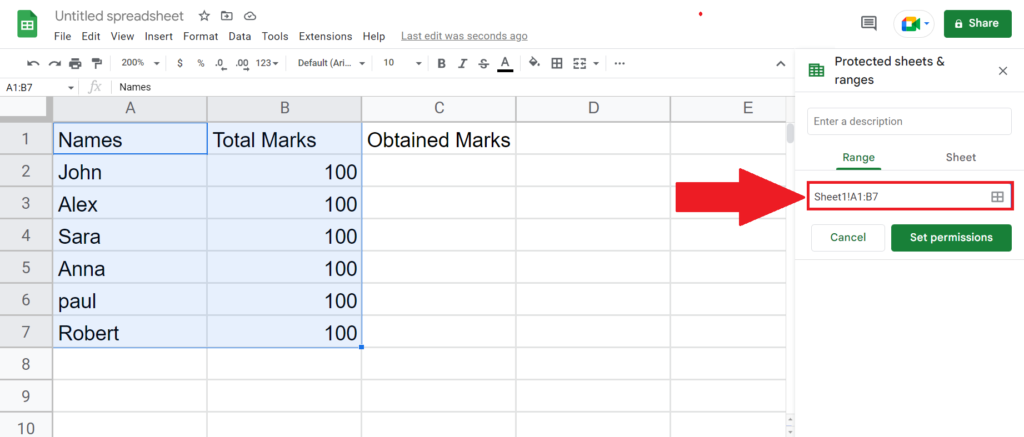
• Enter the range of cells you want to lock.

Step 5 – Click on Set Permissions

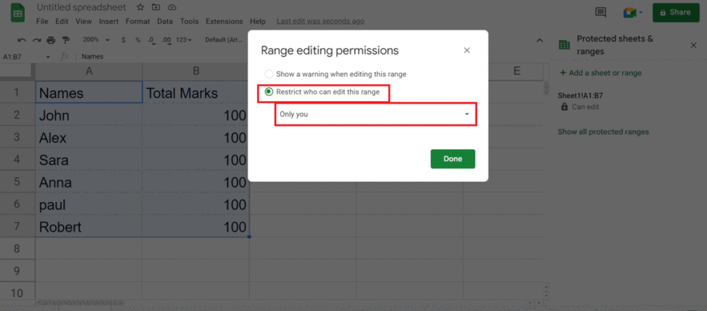
• Click on the Set Permissions option.
• Restrict the range by selecting “Restrict who can edit this range” and selecting “only you”.

Step 6 – Click on Done

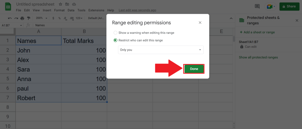
• Click on Done in the Range editing permission option.
• The selected range will be locked and only you would be able to edit it.
• You may customize the restriction and choose who can edit the range.

Method 2: Using the Context Menu to Lock Cells

The same thing can be done by using the context menu as well. 

Step 1 – Right Click Anywhere on the Sheet

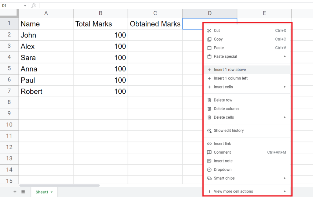
• Right-click on the Sheet.
• The context menu will appear.

Step 2 – Click on the “View more cell actions” Option and Click on the “Protect range” Option

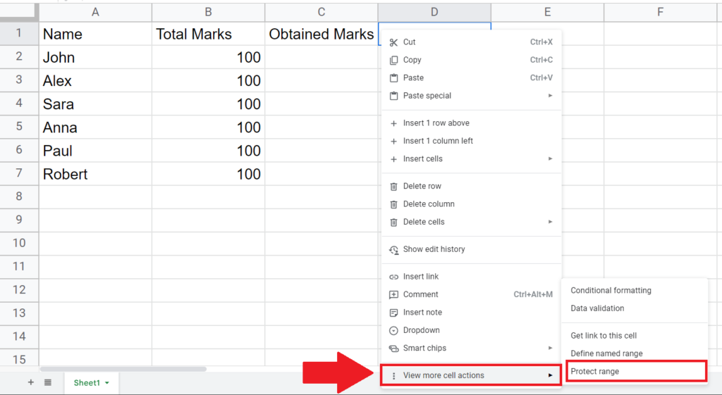
• Click on the “View more cell actions” option in the context menu.
• Click on the “Protect range” Option.

Step 3 – Click on “Add a sheet or Range” 

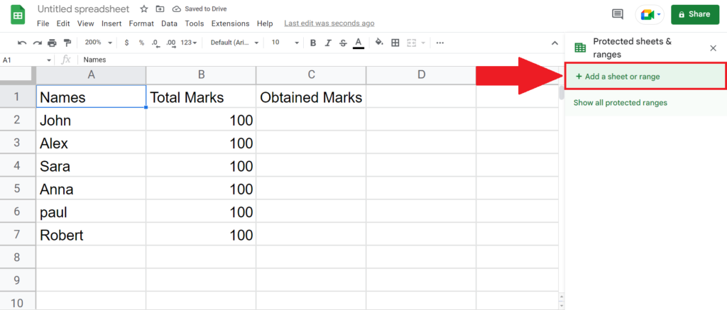
• Click on the “Add a Sheet or range” option.

Step 4 – Enter the Range of the Cells 

• Enter the range of cells or a single cell that you want to lock.

Step 5 – Click on Set Permissions

• Click on the Set Permissions option.
• Restrict the range by selecting “Restrict who can edit this range” and selecting “only you”.

Step 6 – Click on Done

• Click on Done in the Range editing permission option.
• The selected range will be locked and only you would be able to edit it.
• You may customize the restriction and choose who can edit the range.