
How to lock a formula in Google Sheets
 By
SpreadCheaters
By
SpreadCheaters
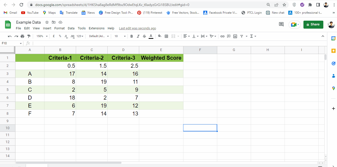
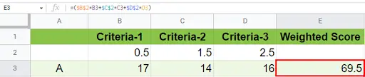
In today’s article, we will learn how to lock a formula in google Sheets. For example, we want to calculate the weighted score given in the following data:

We will be using the formula:
Weighted score = (0.5 * Column B) + (1.5 * Column C) + (2.5 * Column D)
We can lock the weights of each column but we want to have the flexibility of being able to change their weights when needed, thus storing the weights in different cells. We store 0.5 at B2, 1.5 at C2, and 2.5 at D2.
Locking a formula in Google Sheets means that if you have a formula which needs to remain consistent throughout the data, locking it ensures that it remains the same and doesn’t get altered while dragging down the formula, which could result in inaccurate calculations.
Step 1 – Place Equals to (=) sign
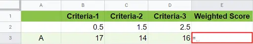
– Start the formula in cell E3 with the equals to the (=) sign.
Step 2 – Add The Formula To A Selected Cell
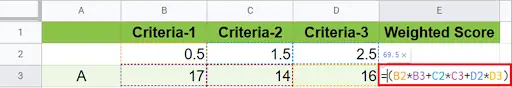
– Now type the formula in the selected cell, which in our case will be;
=B2*B3+C2*C3+D2*D3
Step 3 – Lock the Formula By Adding The Dollar ($) Sign
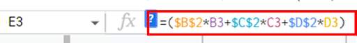
– Start clicking on the formula to add the dollar ($) sign on the cells that should be locked. For our example it should look like this.
=($B$2*B3+$C$2*C3+$D$2*D3)
– The easiest way to add the dollar ($) sign is to click on the formula bar & press the F4 key to add a dollar ($) sign. For this, you should select the required cell addresses which you wish to keep locked or constant through out the data and then press F4.
Step 4 – Press Enter
– Press enter to see the result.
Step 5 – Drag The Formula Downwards

– Copy the formula by dragging it down the cells, you will get the formulas correctly copied and you will notice that the cell addresses of the cells with dollar sign ($) didn’t change though out the data column as shown above.


