
How to label the legend in Google Sheets
 By
SpreadCheaters
By
SpreadCheaters
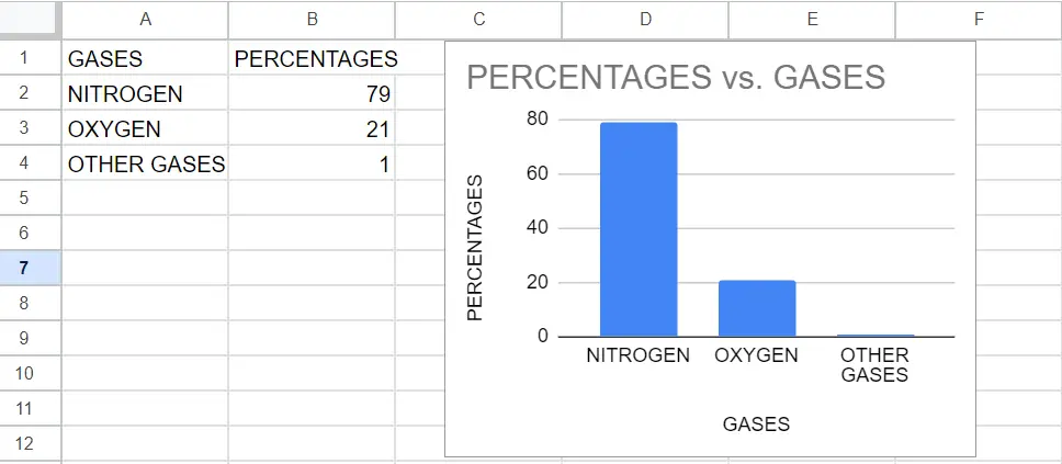
In this tutorial, we will learn how to label the legend in google sheets. In our dataset shown above, we have the percentage of gases in the air and their names in graphical form. Now we want to add labels to legends. For this, we will use the Label option. The following steps will guide you to use this option.

In Google Sheets, a legend is typically used to identify the different series or data sets in a chart. To label, the legend in Google Sheets means to add a title or name to the legend, so that viewers can easily understand which series or data set each color or marker in the chart represents.
Step 1 – Click on the 3 dots symbol
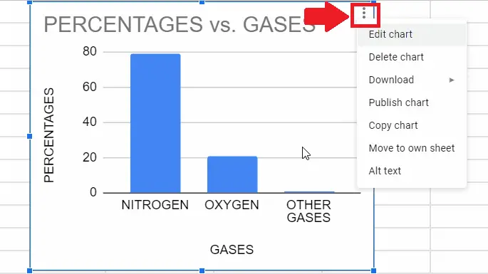
– Click on the 3 dots symbol at the top right corner of the chart and a drop-down menu will appear
Step 2 – Click on the Edit Chart option
– From the drop-down menu, click on the Edit chart menu and a dialog box will appear on the right side of the sheet
Step 3 – Click on the Customize option
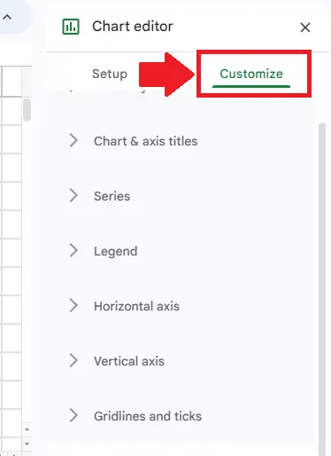
– In the dialog box click on the Customize option at the top of the dialog box and a list of options will appear below in the dialog box
Step 4 – Click on the Legend option
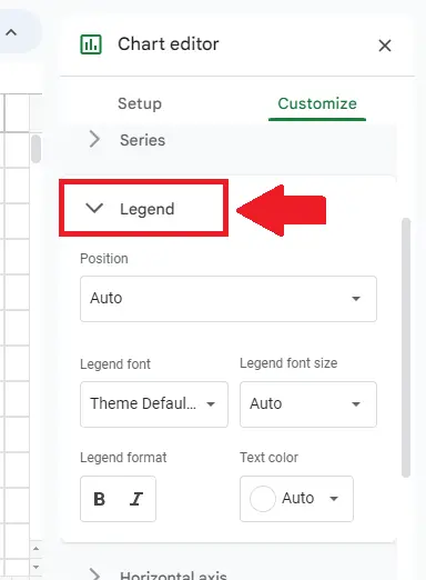
– In the list of the dialog box, click on the Legend option an extended menu will appear
Step 5 – Select the position of Legend
– Select the position of the legend in the box below the position option to get the required result
– Here we have selected Right, you may select any other position


