
How to keep top row visible in Google Sheets
 By
SpreadCheaters
By
SpreadCheaters
The top row freeze feature in Google Sheets allows you to keep the top row visible as you scroll down through your spreadsheet. This can be particularly helpful if you have a large dataset and need to keep the header row visible at all times, as it allows you to quickly reference the column headers without having to scroll back up.
Here are some of the benefits of keeping the top row freeze in Google Sheets:
- Easy Navigation: With the top row freeze, you can easily navigate through your spreadsheet without losing sight of the column headers. This can save you time and effort, especially when you need to work with large data sets.
- Better Organization: The top-row freeze can help you organise your spreadsheet more effectively. By keeping the column headers visible, you can easily see which columns contain which data, making it easier to analyze and interpret your data.
Overall, the top-row freeze is a simple yet powerful feature that can help you work more efficiently and effectively in Google Sheets.
Let’s learn this through an example.
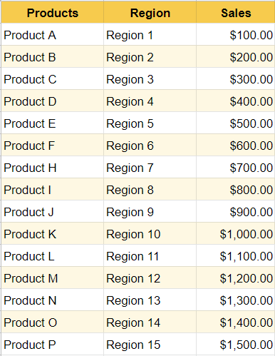
We have the following dataset that needs to be updated daily. To save our time of scrolling up & down, we will freeze the top row / headings for our table with these two methods.
Method 1 – From View Menu
Step 1 – Select Row
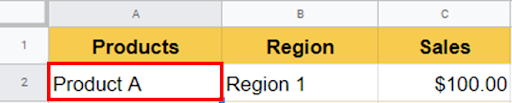
- Place your cursor under the first row i.e row that needs to be frozen.
Step 2 – Go To View Menu
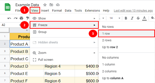
- Go to the view menu.
- Click on the freeze menu.
- Here you will see options to freeze rows & columns. Since we want to freeze the top row, we will select the 1 row option.
Step 3 – Top Row Frozen
- The moment you click on the 1 row option, a thick grey line under your headings will appear which means the top row will be visible all the time you scroll down.
Method 2 – Through Hand Icon
Step 1 – Move Cursor To The Top Left Corner
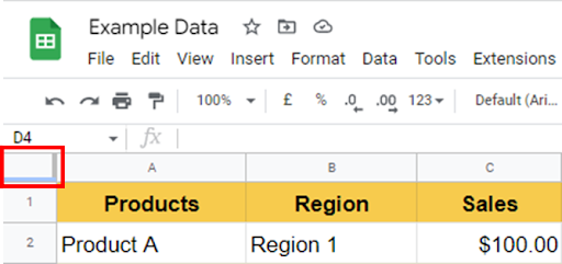
- Move your cursor to the top left corner of your worksheet area. There would be a blank grey box with two thick grey lines as shown below.
Step 2 – Drag the row-freezing border using the mouse
- Hover the cursor over the horizontal grey line. You will notice that the cursor changes to a hand icon.
- Hold the left-mouse key and drag this line down. Since you only want to freeze the top of the row, bring this line just below the first row and leave the mouse key.


