How to keep column width fixed in Excel
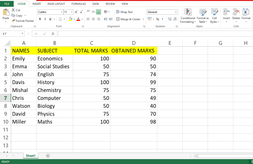
In this tutorial, we will learn how to fix column width in Excel. Consider the following dataset to learn it. The following dataset represents the students’ names, subjects, total marks, and obtained marks. Follow the given steps to learn how to keep column width fixed in Excel. First, we will set the width of the column and then we will lock/fix it.
Fixing the width of a column in Excel means setting a specific width for the column so that its size remains constant, regardless of the content it contains. However, fixing the width allows you to control the appearance and layout of your spreadsheet by ensuring consistent column sizes. Once you have fixed the width of a column, it will no longer automatically adjust when you add or remove content within it. This can be useful when you want to maintain consistent column sizes throughout your spreadsheet or when you want to align data across different columns more precisely.
Step 1 – Select the column
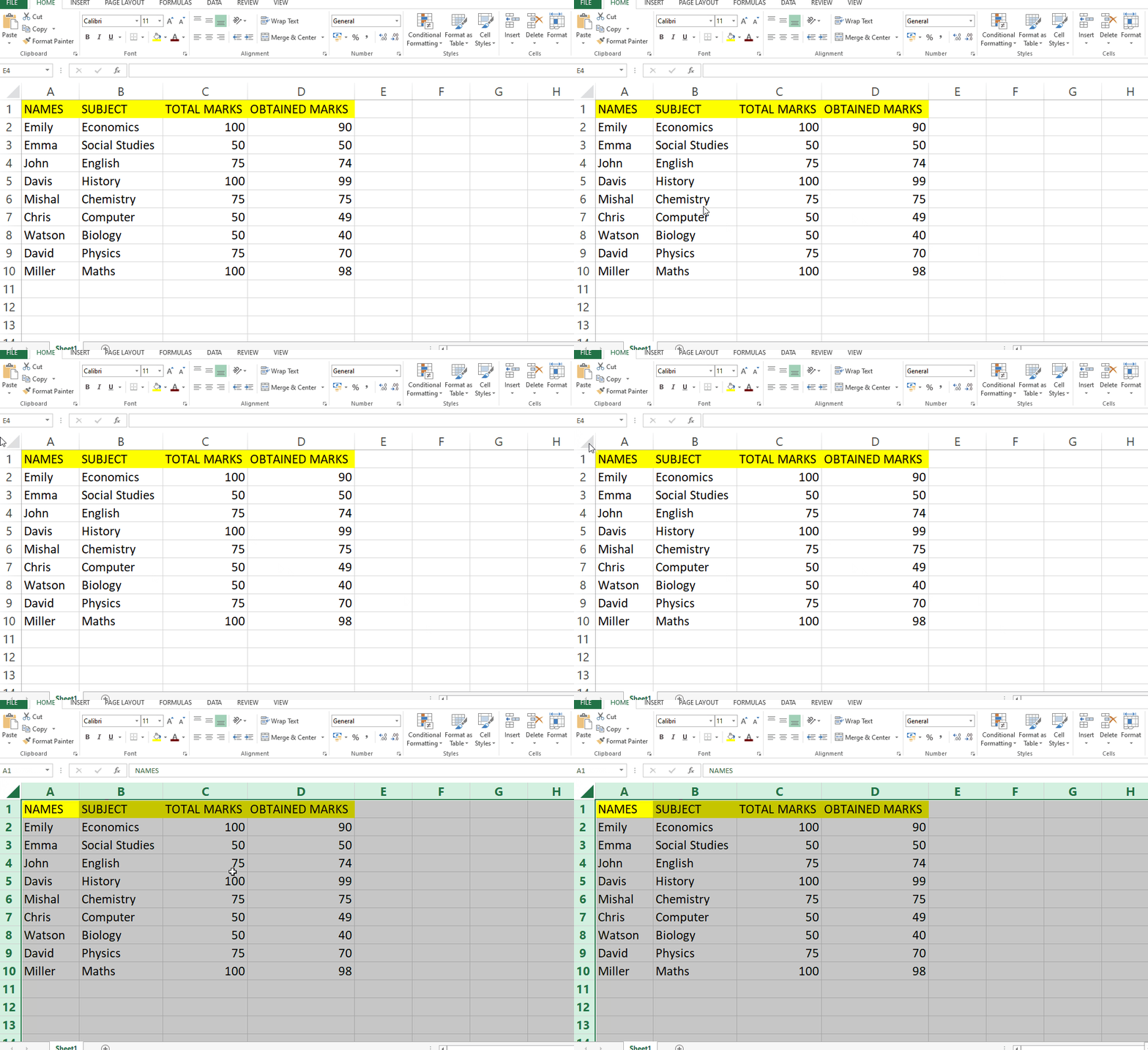
– Select any columns/cells or range of cells.
– In our case, we are selecting all the cells in the sheet.
– You can also do this by clicking on a triangle-shaped icon on the top left corner of the sheet.
Step 2 – Locate the home tab

– For setting an appropriate width of the column, you can go to the home tab.
– Find the cells group, and click on the format button to open a drop-down menu.
Step 3 – Choose column width
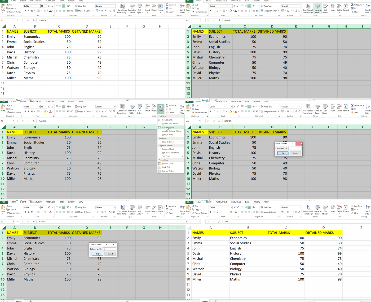
– When you click on FORMAT CELLS, a dropdown menu will appear.
– From that dropdown menu, in the cell size category choose column width.
– Choose the options column width and set an appropriate width for the column.
– We are setting the column to 20.
– Click on OK to confirm setting the width of the column.
Step 4 – Protecting the sheet
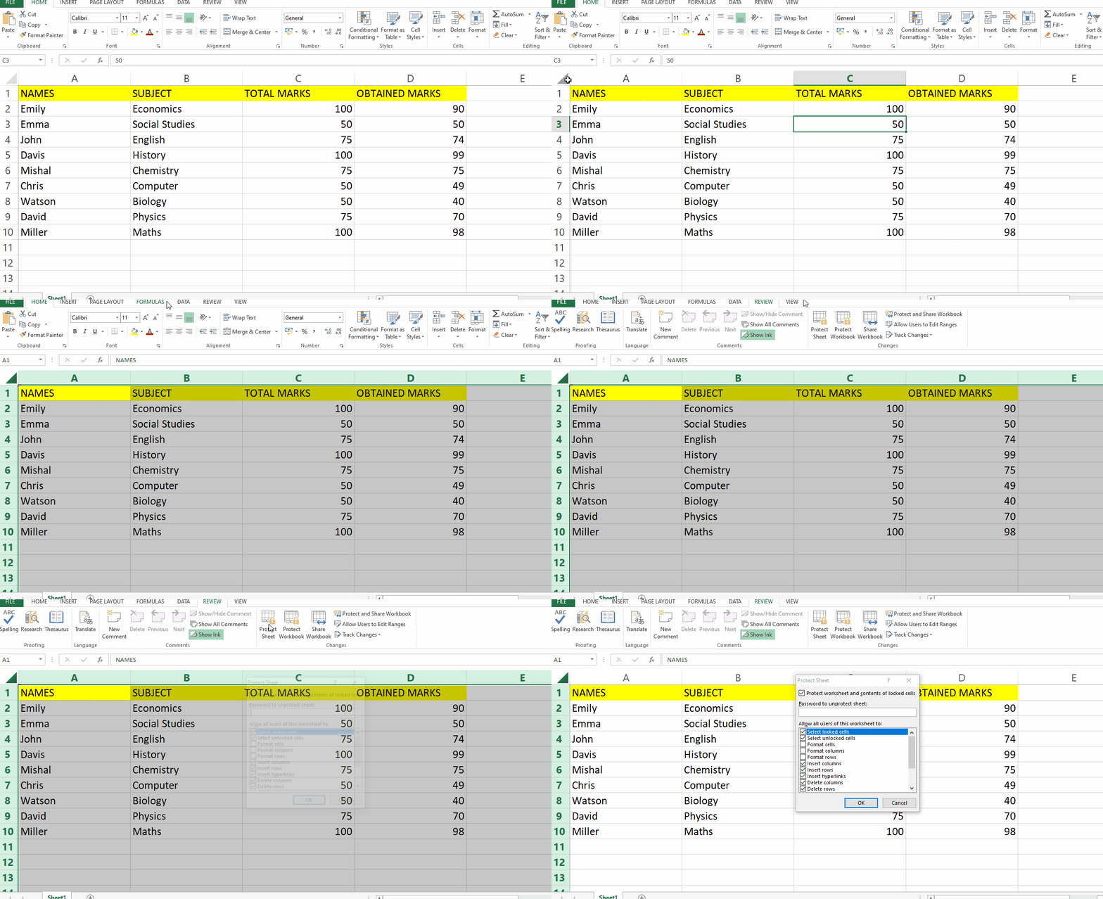
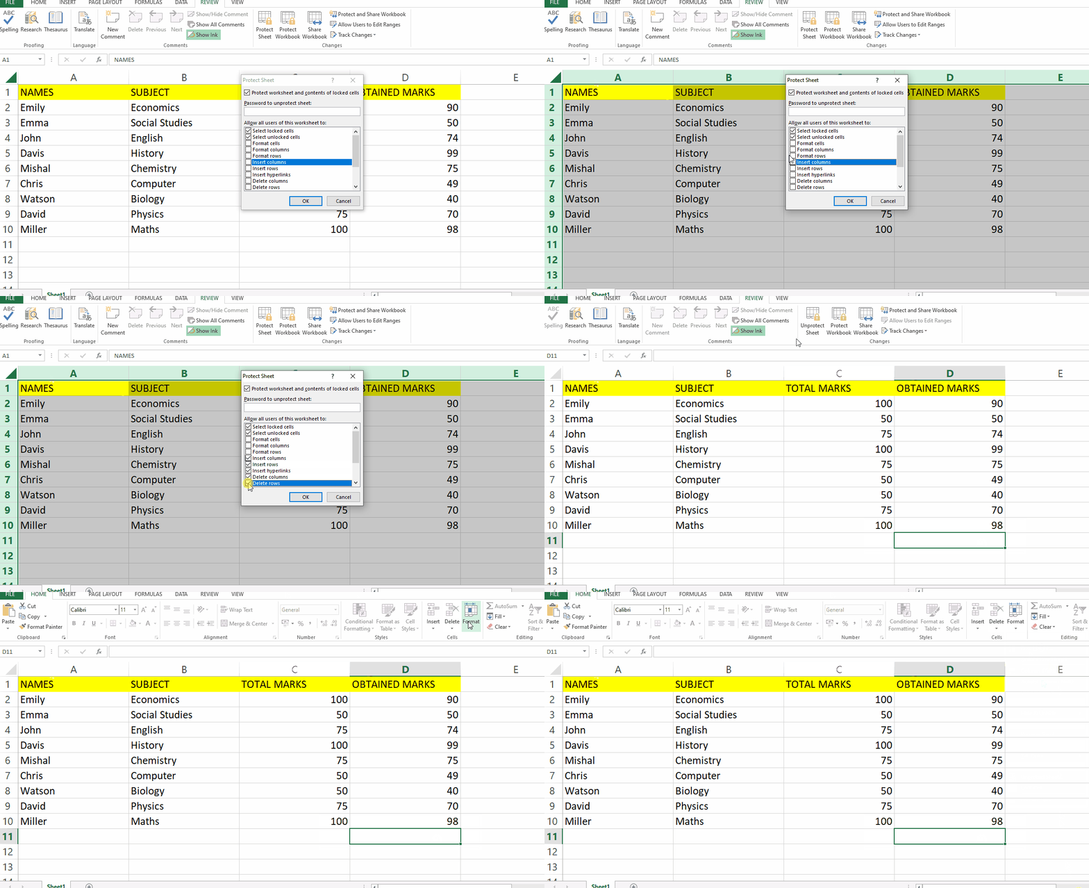
– Now that you have set the column width, for fixing it we need to protect the sheet.
– Go to the review tab, in the Changes group, and select PROTECT SHEET.
– You can enter the password but it’s optional.
– You can enter the password when you are protecting the workbook, in our case we are not doing that.
Step 5 – Check the options

– A, a “protect sheet” dialogue box will appear when you click on the protect sheet option.
– Check the options you want to check.
– In our case we are not checking the options; format cells, format columns, and format rows, because by not checking those options we can perform basic operations like inserting a formula, etc.
– Click on OK to confirm protecting a sheet.
– Now you can see that when go to change the width of the column, the option is disabled, which means that the column width is fixed and you cannot change it now.


