How to hide field headers in PivotTable
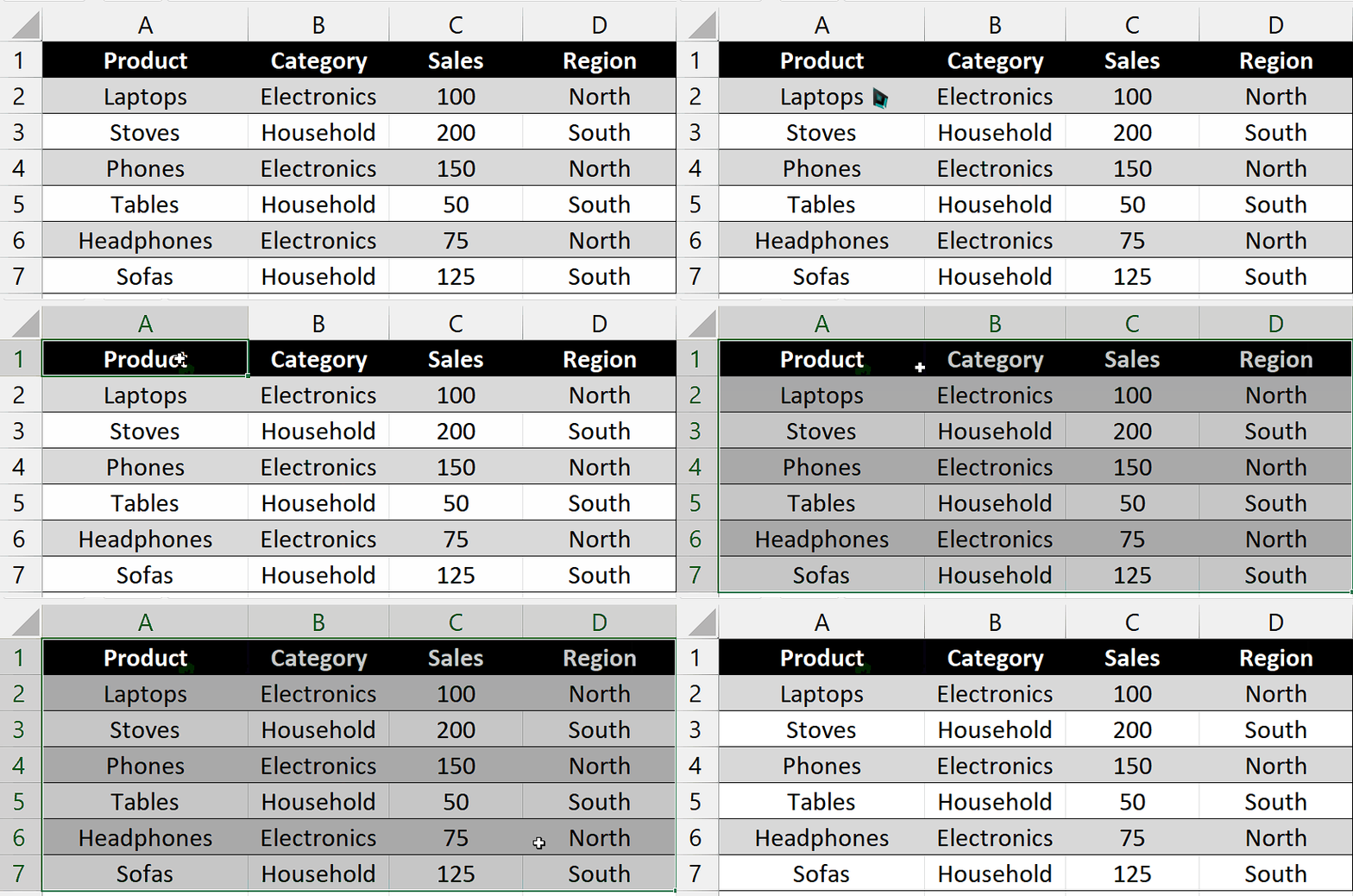
Today’s tutorial focuses on a dataset showcasing sales figures for different product categories in two regions: North and South. The data includes sales breakdowns for the Electronics and Household sectors. The dataset comprises six rows representing specific products, such as Headphones, Laptops, Phones, Sofas, Stoves, and Tables. Each product category is accompanied by its respective sales amount in the Electronics and Household columns. In this tutorial, we will explore how to convert a range into a Pivot Table and demonstrate the process of hiding Field headers within the PivotTable.

Hiding field headers allows you to focus on the summarized data and the visual representation of the pivot table without the distraction of field names. This can make the pivot table more visually appealing and less cluttered, especially when you have multiple fields in the pivot table.
Step 1 – Choose the cell range

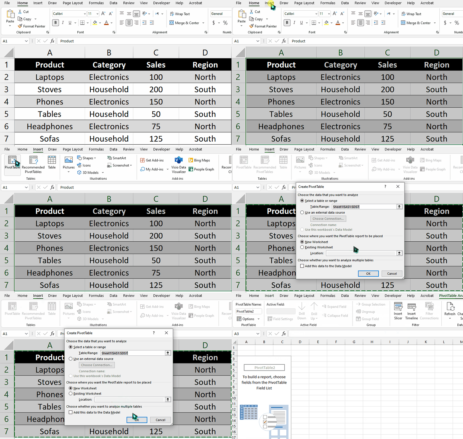
– Begin by selecting the cell range that you wish to convert into a Pivot Table.
– For instance, let’s say we have chosen the cell range “A1:D7” as our data range.
Step 2 – Convert to PivotTable

– Navigate to the “Insert” tab located on the Excel ribbon, where you will find the “PivotTable” command button.
– Click on the command button to open the PivotTable wizard.
– Inside the PivotTable wizard, you will notice that the selected range is already entered in the “Select a table or range” field, reflecting the range of cells you previously selected. Verify that the correct range is displayed and make any necessary adjustments.
– Choose the desired location for your Pivot Table. You have two choices:
New Worksheet: This option generates a new worksheet and positions the Pivot Table there.
Existing Worksheet: Select cells within an existing worksheet where you want the Pivot Table to be inserted.
– Once you have made your selection, click “OK” to proceed.
Step 3 – Construct the PivotTable

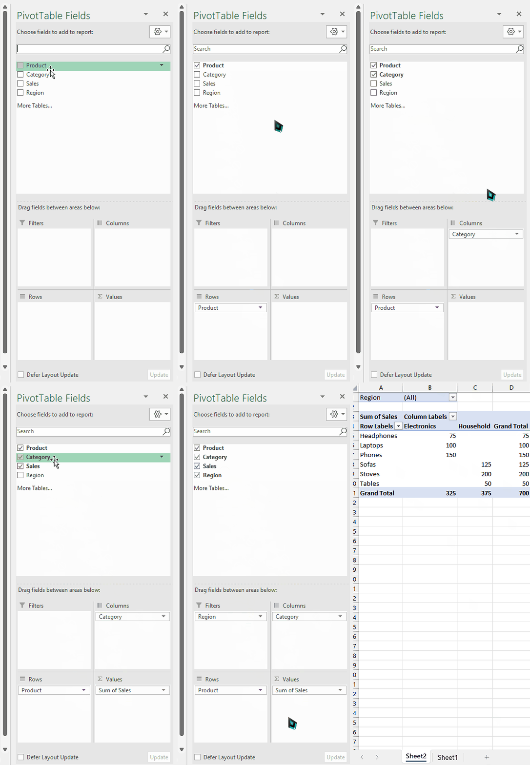
– On the right side of the screen, you will find the PivotTable Field List.
– This field list displays the column headers from your selected date range.
– To begin constructing your PivotTable, drag and drop the desired fields from the field list into four designated areas: Report Filter, Column Labels, Row Labels, and Values.
– To use a specific field as a filter for the entire PivotTable, select and drag it from the PivotTable Field List into the “Report Filter” area. For example, we can choose “Region” as the “Report Filter.”
– For the column headers in the PivotTable, select the appropriate field and drag it into the “Column Labels” area. Let’s say we want to use “Category” as the “Column Label.”
– Next, select the field to be used as row headers in the PivotTable and drag it into the “Row Labels” area. For instance, we can choose “Products” as the “Row Label.”
– Indicate the field that contains the data to be summarized in the PivotTable by dragging it into the “Values” area. In this case, we will enter the “Sales” field in the “Values” area.
– Once you have successfully placed all the necessary fields into their respective areas, your PivotTable will be automatically constructed.
Step 4 – Hide the Field Headers

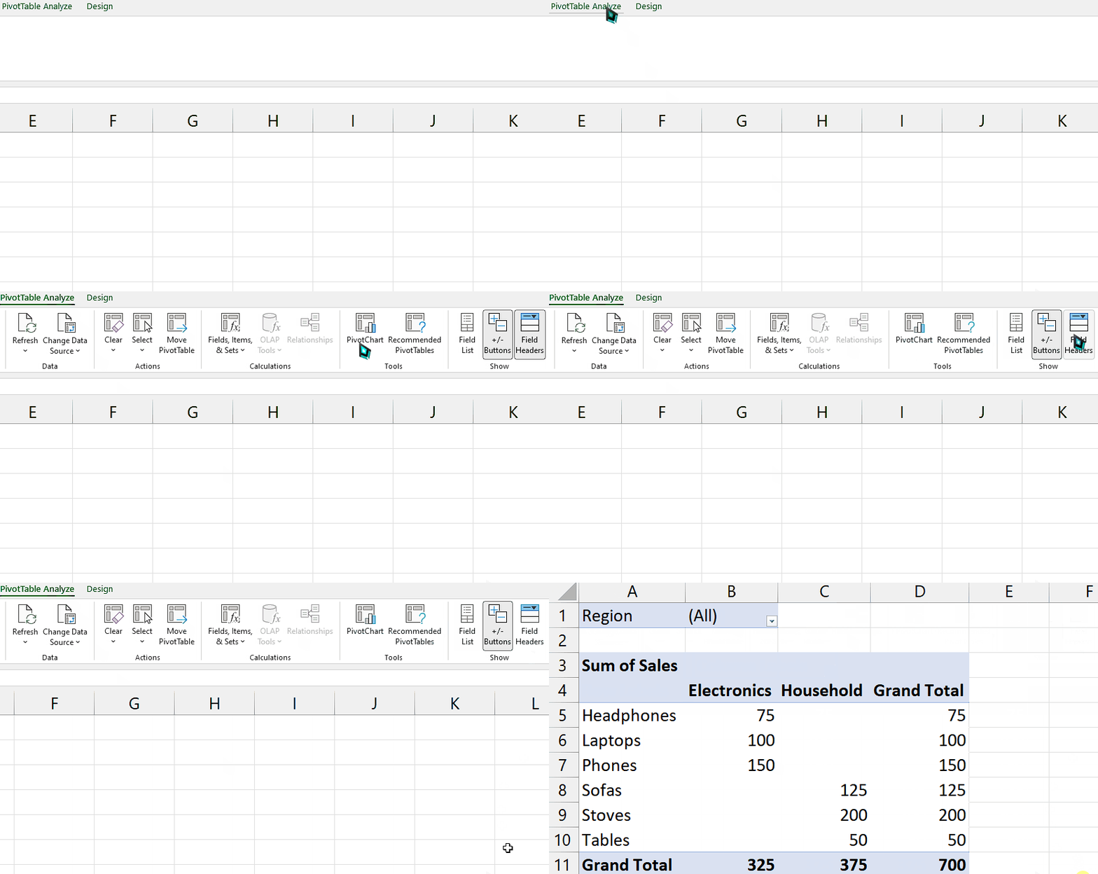
– In the current state, our PivotTable displays Field Headers labeled as “Column Labels” and “Row Labels” by default.
– To hide these Field Headers, go to the “PivotTable” Analyze tab.
– Within the “Show” group, locate the “Field Headers” command button.
– Click on the “Field Headers” command button, and the Field Headers will be hidden from view.
Alternatively, you can press the “Alt Key” and then press the “J key” with the “T key” to open the “PivotTable” Analyze tab.
– Then, press the “H key” to hide the Field Headers.


