
How to flip columns and rows in Google Sheets
 By
SpreadCheaters
By
SpreadCheaters
Flipping columns and rows in Google Sheets means transposing the data in a given range so that the columns become rows and the rows become columns. Flipping columns and rows in Google Sheets can be an important tool for organizing, analyzing, and presenting data in a way that makes it easier to understand and use.
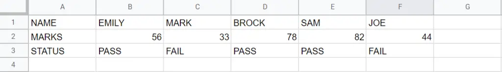
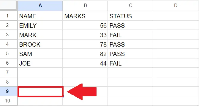
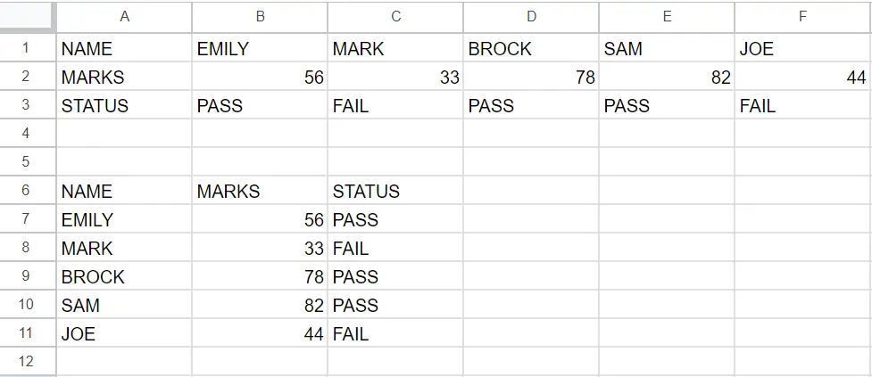
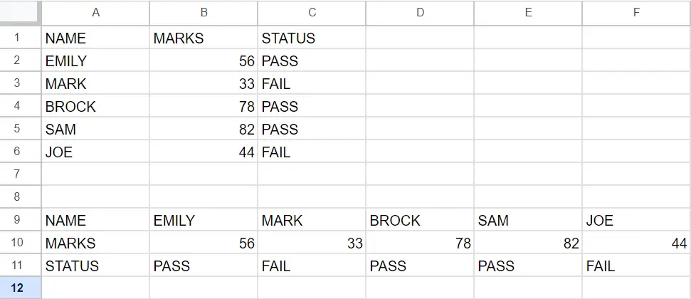
In our data set, the names of students written with their marks and educational status are shown. Now we want to flip the data, for this, we will first copy the data and then use the Paste Special function. The following steps will guide you to use this option.
Method 1: Flip the Rows Using the Paste Transpose option
Step 1 – Select the Range of Data
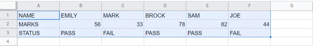
- Select the range of cells to be flipped by using drag and drop method
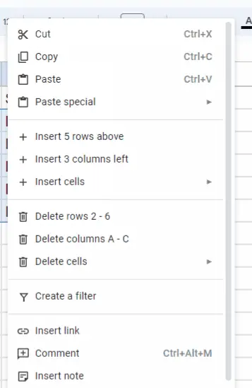
Step 2 – Open the Context menu
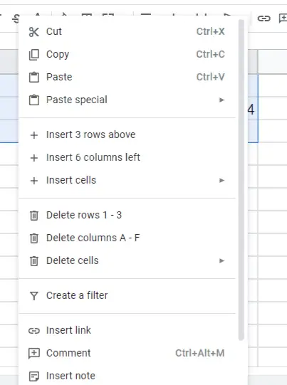
- Right-click anywhere in the selected range of cells to open the context menu
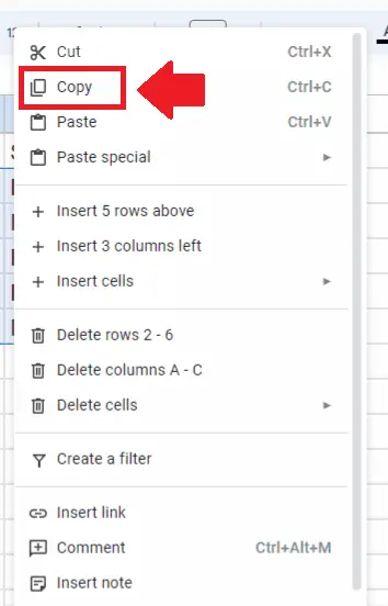
Step 3 – Copy the Data
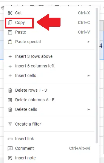
- In the context menu, click on the Copy option
Step 4 – Select the Cell
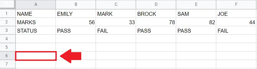
- Click on the cell where you want to show the flipped data
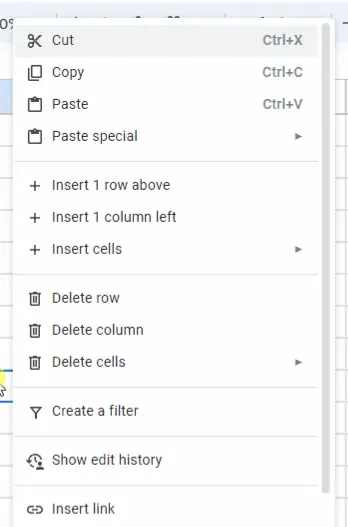
Step 5 – Open the Context menu
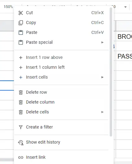
- Right-click in the selected cell to open the context menu
Step 6 – Click on Transposed
- In the context menu, Click on the arrow next to the Paste Special option and a right-side menu will appear
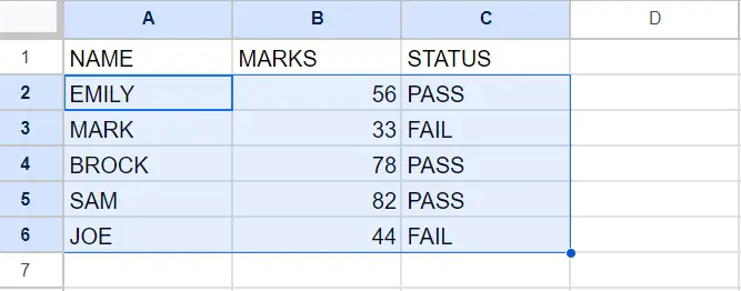
- From this menu, Click on Transposed to get the required data
Method 2: Flip the Columns Using the Paste Transpose option
Step 1 – Select the Range of Data
- Select the range of cells to be flipped by using drag and drop method
Step 2 – Open the Context menu
- Right-click anywhere in the selected range of cells to open the context menu
Step 3 – Copy the Data
- In the context menu, click on the Copy option
Step 4 – Select the Cell
- Click on the cell where you want to show the flipped data
Step 5 – Open the Context menu
- Right-click in the selected cell to open the context menu
Step 6 – Click on Transposed
- In the context menu, Click on the arrow next to the Paste Special option and a right-side menu will appear
- From this menu, Click on Transposed to get the required data
Method 3: Flip the Rows Using the Transpose function
The TRANSPOSE function “flips” the orientation of a given range or array: TRANSPOSE flips a vertical range to a horizontal range and flips a horizontal range to a vertical range.
Syntax of the Transpose function is:
=TRANSPOSE(array)
- The array argument is a range of cells to be flipped.
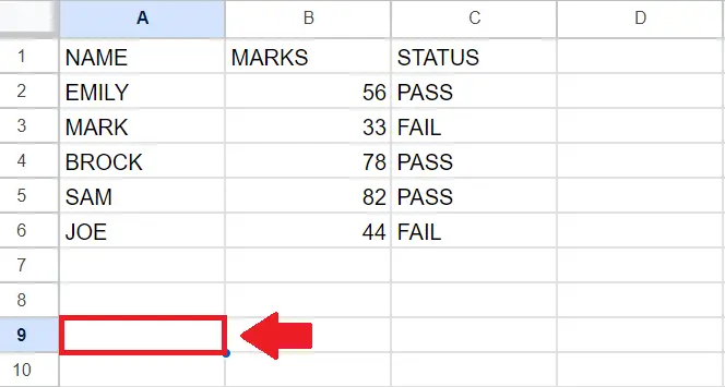
Step 1 – Select the cell
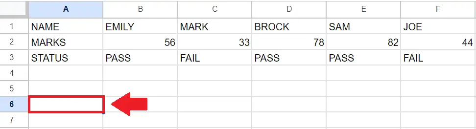
- Click on the cell, where you want to show the vertical data
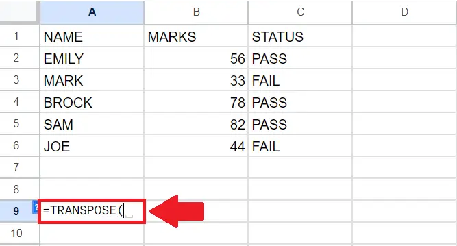
Step 2 – Use the Transpose function
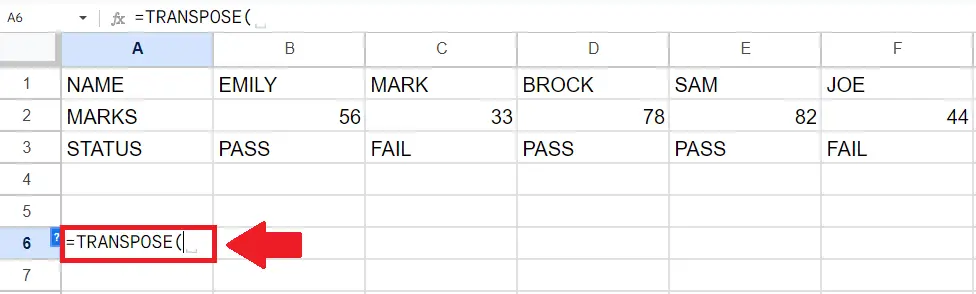
- To use the transpose function, type “=Transpose(” in the selected cell
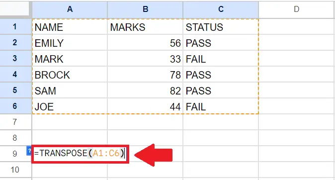
Step 3 – Type the Argument of the function
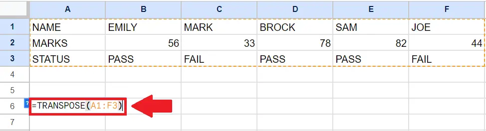
- Type the argument of the Transpose function(array)
- array: A1:F3
- After typing the argument, type the closing bracket “)”
Step 4 – Press the Enter key
- After typing the argument, press the Enter key to get the required result
Method 4: Flip the Columns Using the Paste Transpose function
The TRANSPOSE function “flips” the orientation of a given range or array: TRANSPOSE flips a vertical range to a horizontal range and flips a horizontal range to a vertical range.
Syntax of the Transpose function is:
=TRANSPOSE(array)
- The array argument is a range of cells to be flipped.
Step 1 – Select the cell
- Click on the cell, where you want to show the horizontal data
Step 2 – Use the Transpose function
- To use the transpose function, type “=Transpose(” in the selected cell
Step 3 – Type the Argument of the function
- Type the argument of the Transpose function(array)
- array: A1:C6
- After typing the argument, type the closing bracket “)”
Step 4 – Press the Enter key
- After typing the argument, press the Enter key to get the required result


