
How to find curved line equations in Excel
 By
SpreadCheaters
By
SpreadCheaters
In this article, we will learn how to show curved line equations in Microsoft Excel. Mainly the Trendline feature in Microsoft Excel is utilized to show the curve line equation.
Let’s say we have temperature readings at different time stamps. We aim to show the curved line equation of the readings.
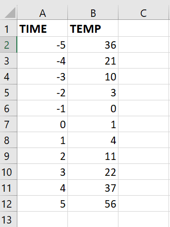
In Excel, a curved line equation refers to the mathematical equation that represents a curved line on a graph or chart. It is used to calculate the values of the y-coordinate (dependent variable) corresponding to different x-coordinate (independent variable) values along the curve.
Step 1 – Select the range of cells
– Select the range of cells for which you want to form the curve
Step 2: Click on the Insert Scatter or Bubble Chart option
– Click on the Scatter or Bubble Chart option from the Charts group of the Insert tab and the drop-down menu will appear
Step 3 – Click on the Scatter chart
– From the drop-down menu, click on the Scatter graph to select it
– And a Scatter chart will appear on the sheet
Step 4 – Right click on the Data Series
– After the chart appears on the sheet, right-click on any Data series and a context menu will appear
Step 5 – Click on the Add Trend Line option
– From the context menu, click on the Add Trend Line option and a dialog box will appear on the right side of the sheet
Step 6 – Select the data to be shown on the graph
– From the dialog box Tick the check box of Display the Equation on the Chart option
– Also, tick the check box of the Display R squared value on the chart option
Step 7 – Choose Polynomial Trendline Option
– In the trendline options, choose the option labeled “Polynomial”.
– We have to select the option that displayed the highest R squared value i.e. for a polynomial it is “0.991”.


