
How to use exponential trendline in Excel
 By
SpreadCheaters
By
SpreadCheaters
In this tutorial we will learn to form an exponential trendline. To add an exponential trend line in Excel, you first need to create a chart that displays the data you want to analyze. Once the chart is created, you can add the trend line. Following are the steps that guide how to add an exponential trend line.

In Excel, an exponential trend line is a type of trend line that can be added to a chart to display the trend of data that follows an exponential pattern. An exponential trend line is useful when the data is changing at an increasing or decreasing rate and follows a curve that can be modeled by the exponential function.
Step 1 – Select the range of cell
– Select the Range of cell for which you want to show trend line
Step 2 – Click on Dialog launcher
– Click on dialog launcher of charts in Insert tab and a dialog box will appear
Step 3 – Select the Chart
– From the drop down menu click on All Charts
– Click on Column
– After clicking column, Column charts will appear
– Select the second chart
– Click on OK to get the graph on sheet
Step 4 – Click on Chart Elements option
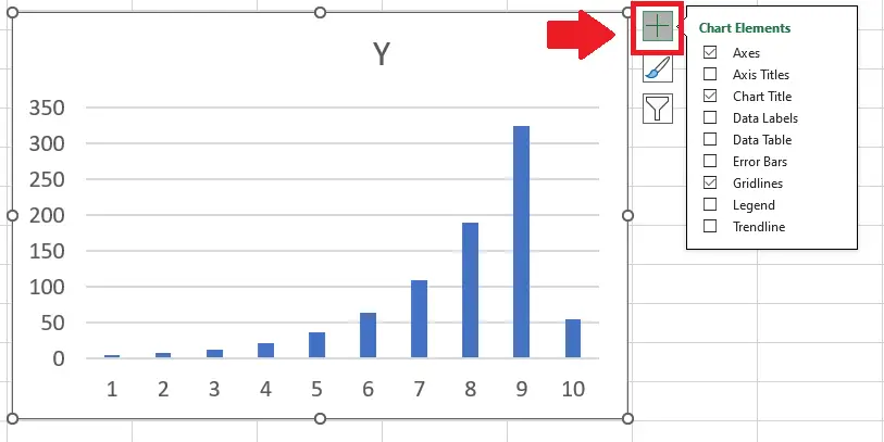
– Click on Chart Elements option at the top right of the graph and a dropdown menu will appear
Step 5 – Click on Trendline
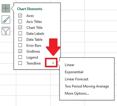
– From the dropdown menu click on Arrow next to Trendline option and a drop down menu will appear
Step 6 – Click on Exponential
– From the dropdown menu click on Exponential to get the required result


