How to filter strikethrough in Excel 

Filters in Excel allow you to selectively display or hide data based on specific conditions. By applying filters, you can focus on specific data subsets, sort data, or hide irrelevant information. For example, you can filter data to display only the sales figures for a particular region or to hide rows with negative values. 

To filter strikethrough text in Excel, you can use different methods. Here’s a step-by-step guide for each method: 

Method 1 – Using the find and replace option 

This method allows us to filter strikethrough in Excel by MS Excel’s built-in tool of find and replace. In this method, we first color the strikethrough data with a specific color of your choice. In fact, there is no direct method to filter the strikethrough data. Hence, we use a customized method to make it happen. The steps are given below; 

Step 1 – Color the strikethrough data 

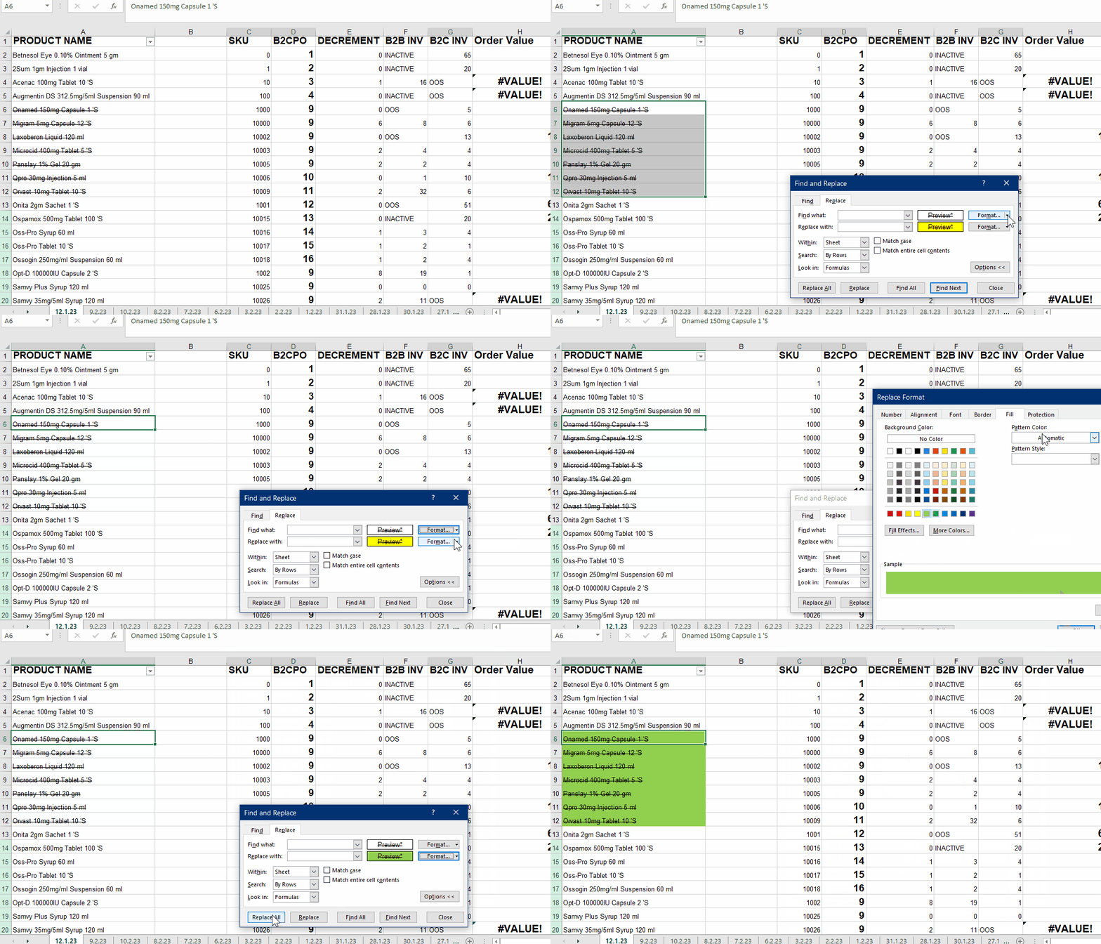
• Open the Excel sheet. 
• Select the strike-through data.  

• Go to the home tab and at the right corner of the icon bar. 
•  Click on the find and select. 
• Click on replace. Or press CTRL + H. 
• Find and replace the dialogue box will. 
• Go to Replace tab, click on the format button of find what: 

• A dropped menu will appear. 
• Click on Choose format from the cell. 
• Pick the cell with the help of a picker. 
• Click on the format button to replace with. 
• A formatting dialogue box will open. 

• Go to the Format tab, and select the color that you want to add in strike-through data cells. 
• Click OK.  
• Click on Replace All. All the strikethrough data will be colored. As shown below; 

Step 2 – Apply the filter  

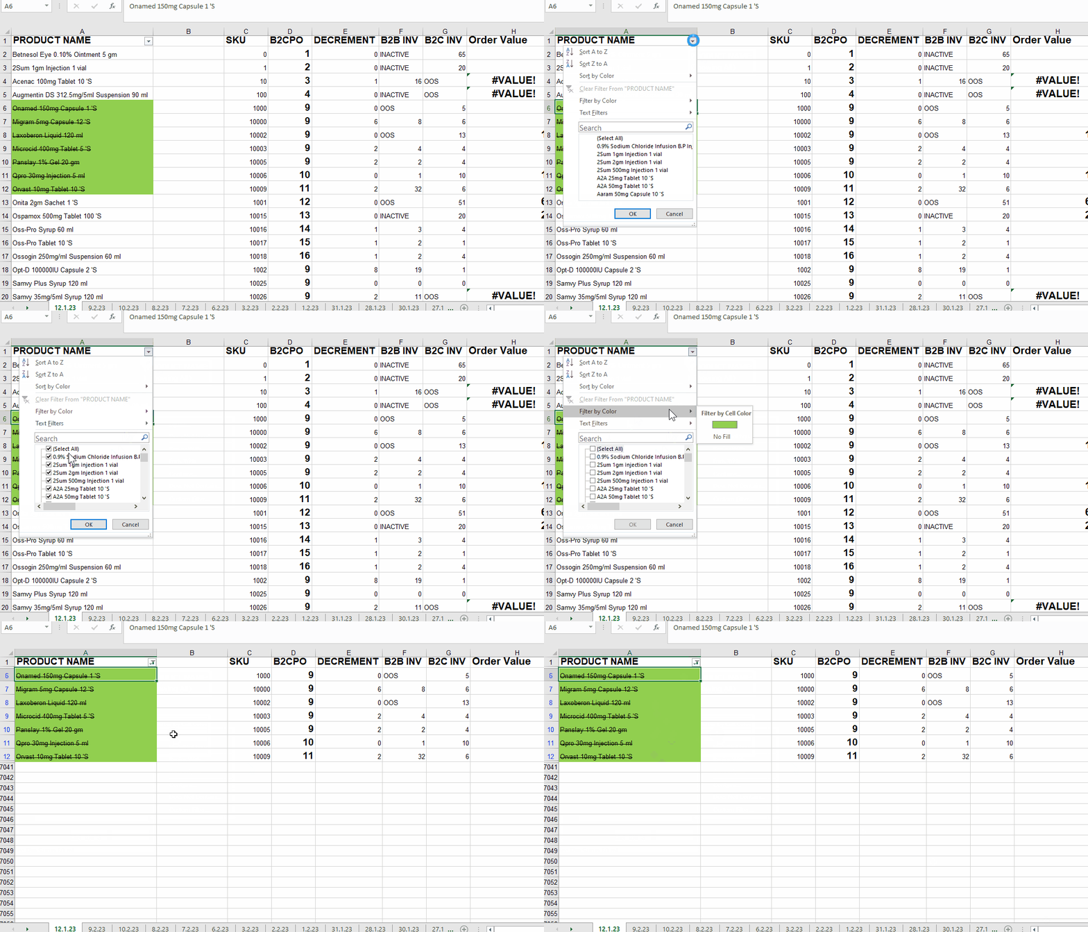
• Press the CTRL + SHIFT + L  to apply the filter on the top row of the sheet. 
• Click on the dropdown icon on the right side of the column name. 
• Drop down menu will appear with certain conditions. 
• Click on the filter by color. 
• A side menu will appear. Click on the color of the strikethrough data cells. 

• All the strikethrough data cells will be filtered. As shown below; 

Method 2 – Using VB code  

In this method, we will use a VB code to filter out the strikethrough data cells, by mentioning a true or false beside every cell. 

Here is a simple code by which we make an Excel boolean function of =HasStrike. Which will result in TRUE or FALSE after checking the cell. The code is  

Function HasStrike(Rng As Range) As Boolean 
   HasStrike = Rng.Font.Strikethrough 
End Function 

 The steps are given below ; 

Step 1 – Open the file and go to the VBA code segment 

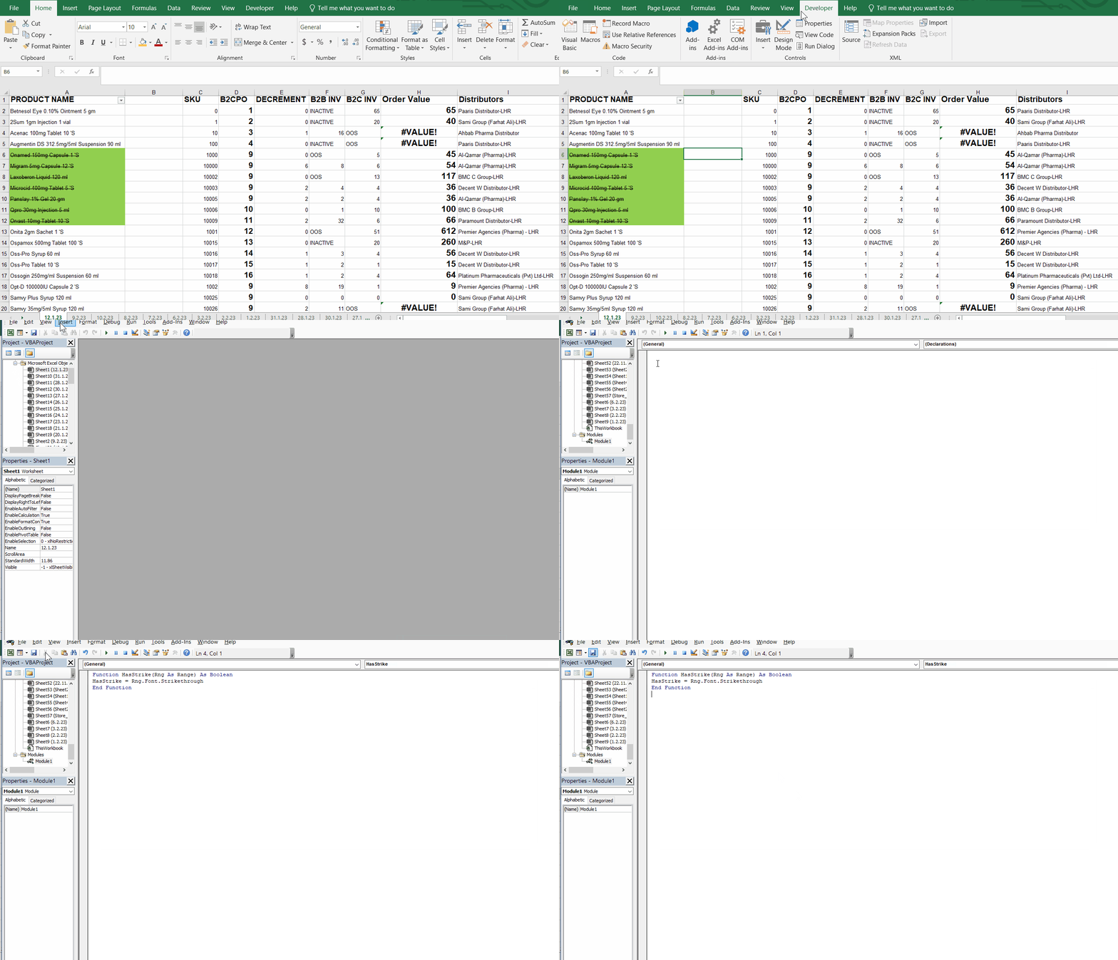
• Open the Microsoft Excel file in which you want to filter strikethrough data. 
• Go to the Developers Tab. Click on the VISUAL BASIC in the CODE cluster. 
• A new window of visual basic code will open. 

• Go to the Insert tab, a drop-down menu will appear. 
• Click on the MODULE. 
• A white blank window will open. 
• Paste the above-mentioned code there. 
• Press CTRL + S or press the save button in the icon bar. Animation is shown below; 

Step 2 – Apply the function  

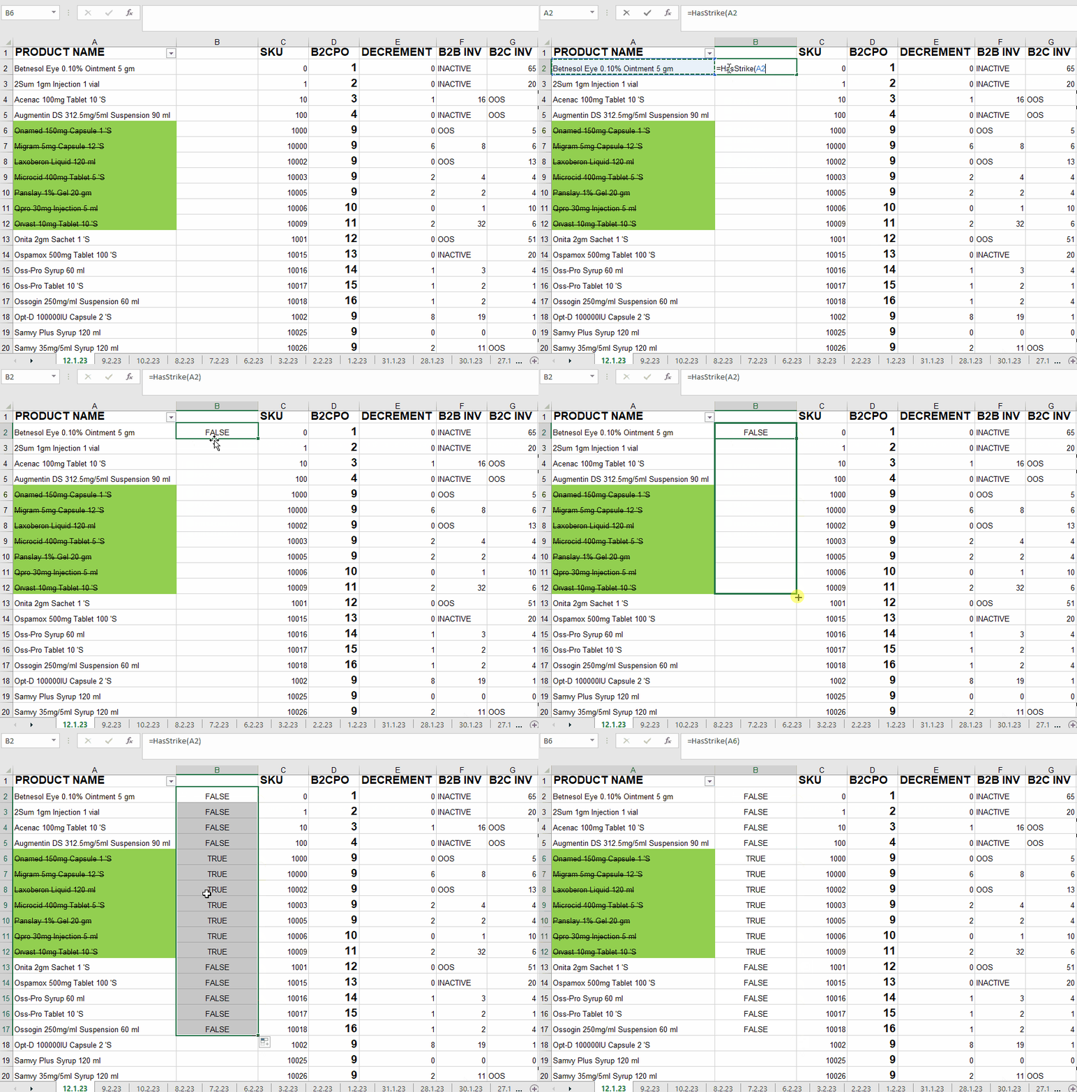
• Add an empty column at the right side of strikethrough data cells. 
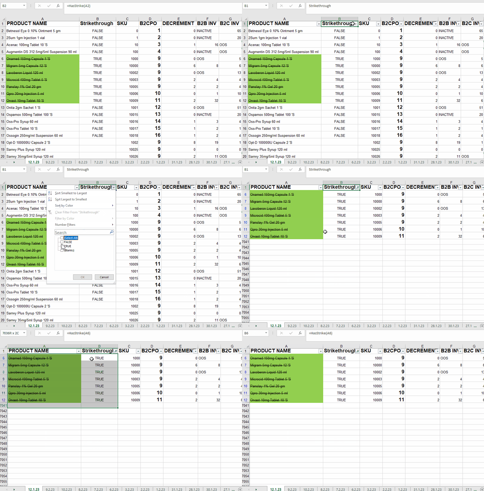
• Apply the function, in this case, we have =HasStrike(B2). 
• As soon as you press the enter key, if the reference cell has strikethrough data, it will return the value as TRUE. 
• if the reference cell has no strikethrough data, it will return the value as FALSE. 

• Drag the result till your data range with the help of filler. As shown below; 

Step 3 – Apply the filter 

• Once you are done with finding the strikethrough data. 

• Press the CTRL + SHIFT + L  to apply the filter on the top row of the sheet. 
• Click on the dropdown icon on the right side of the column name. 
• Drop down menu will appear with certain conditions. 
• Uncheck all the options and mark a tick on TRUE. 
• Click ok.