How to filter data Horizontally in Excel

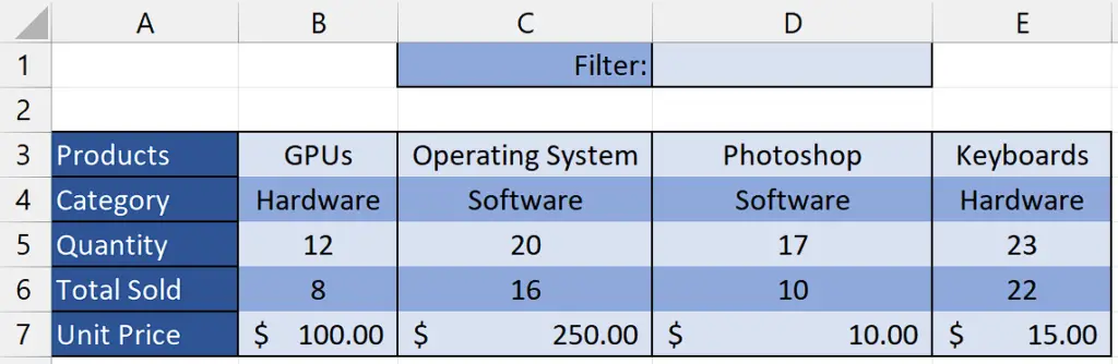
The given data represent different product categories and their corresponding attributes, such as the quantity, total sold, and unit price. Filtering data horizontally by “Hardware” allows us to focus solely on the hardware-related products, namely GPUs and Keyboards. This enables a targeted analysis and comparison of the hardware category’s specific metrics, aiding in decision-making and performance evaluation. In today’s tutorial, we will learn how to filter data horizontally by taking this dataset as an example.

Understanding the function and its syntax

FILTER Function:

In Excel, the FILTER function is used to extract specific data from a range or table based on specified criteria. Its syntax is as follows:

Here is the breakdown of the formula:

array: This is the range or table from which you want to filter the data.

include: This is the criteria or conditions that the data must meet to be included in the result. It can be a range, an expression, or a logical condition.

[if_empty] (optional): This parameter is used to specify the value or action to be taken if no data meets the specified criteria. It is an optional parameter.

Filtering data horizontally in Excel allows you to selectively display or analyze specific columns of data while hiding the others. It helps in focusing on particular attributes or variables of interest and facilitates data exploration, comparison, and decision-making based on specific criteria.

Step 1 – Write the name of the filter 

– Select any empty cell and enter the name of the filter you would like to use for data filtering.
– For example, we have written “Hardware” in the cell D1.

Step 2 – Select the cell

– Select any empty cell where you would like the horizontally filtered data to be displayed.
– In this cell, we will apply the “FILTER” Function to filter the data horizontally.

Step 3 – Write and implement the formula

– Write the following formula in the selected cell
=FILTER(B3:E7, B4:E4=D1, “Not Found”)
Where;
B3:E7: This is the range of data you want to filter. It represents the cells from B3 to E7.

B4:E4=D1: This is the filtering criteria. It specifies that you want to filter the data where the values in cells B4 to E4 are equal to the value in cell D1.

“Not Found”: This is the optional value you want to display if the filter does not find any matching data. In this case, if no matching data is found, it will display “Not Found”.

– After writing the formula, press “Enter” and your data will be filtered horizontally.