
How to filter by color in Google Sheets
 By
SpreadCheaters
By
SpreadCheaters
In this tutorial we will learn how to filter by color in Google Sheets.Performing a color-based filter is a frequently used function in Google Sheets, which can be accomplished through the utilization of the “Filter By Color” option available in the context menu.
Currently we have a data set showing some products and their discounted prices. We aim to filter out the products that are discounted using filter by color.

Google Sheets’ “Filter by color” function is a valuable feature that facilitates the visual arrangement and examination of data via color-coding. This feature enables users to effortlessly filter and arrange data by taking into consideration the background or font color of cells. It proves to be an extremely beneficial tool for monitoring progress, recognizing patterns, highlighting crucial information, and more.
Step 1 – Highlight the Data using Fill Color Button
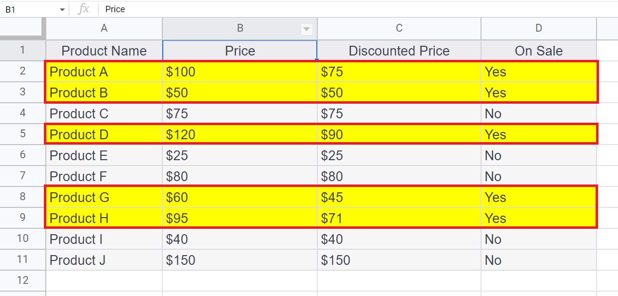
– Highlight the data to be filtered out by the Fill color button.
– Here we have highlighted the discounted products using the yellow color.
Step 2 – Select the Data
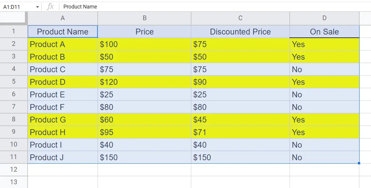
– Select the data containing the data to be filtered by color.
Step 3 – Click on the Create a Filter Button
– Click on the Create a Filter button in the ribbon.
– Filter options will appear right next to each column header of the selected data.
Step 4 – Click on one of the Filter Options
– Click on any of the filter options right next to the headers.
– A drop-down menu will appear.
Step 5 – Click on the Filter by color Option and
– Click on Fill color
– Click on the Filter by color option in the drop-down menu.
– Then click on the Fill color option.
Step 6 – Click on the Color
– Select the color of the highlighted data to filter the data by color.
– The data will be filtered by that color.


