How to filter a pivot table with a custom list.

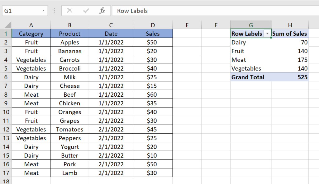
Here we have a pivot table, in which there is the Sum of Sales of four categories Meat, Vegetables, Fruit, and Dairy. In this tutorial, we will understand how to filter a pivot table in Excel but first let’s take a look at the Dataset.

Method – 1 Using Slicer

Slicers in Excel are visual controls that allow you to filter and interact with data in a pivot table. They provide a user-friendly way to filter data without the need to use complex filter options or modify the underlying pivot table structure.

Filtering a pivot table in Excel with a custom list is useful for analyzing specific data within your larger dataset. By using a custom list, you can filter the pivot table to show only the data that you want.

Step – 1 Insert Slicer.

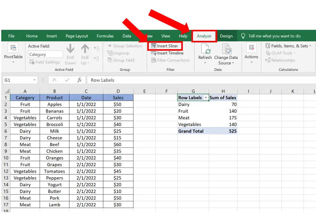
– Select any cell inside the Pivot Table.
– Go to the Analyze tab.
– In the Filter group click on the Insert Slicer command.

Step – 2 Filter the values

– Clicking on the Insert Slicer command will reveal the Insert Slicer dialog box.
– Select the categories you want the slicer to display.
– The filter criteria will be displayed 
– You can filter the Pivot Table by filtering out multiple items and see the result varying in value areas.