
How to filter pivot table values in Microsoft Excel
 By
SpreadCheaters
By
SpreadCheaters
In this tutorial we will learn how to filter pivot table values in Microsoft Excel.Filtering PivotTable values in Excel is a straightforward process that can be accomplished in just a few simple steps.To filter pivot table value we use the drop down arrow right next to the column headers in the pivot table.
Right now we have a pivot table showing the sales of some products in different regions and months. we aim to filter the figures for the Product D and F.

Filtering PivotTable values is a powerful feature in Excel that can help you analyze, present, and understand large datasets more effectively. Whether you are a data analyst, business professional, or student, this feature can help you make better decisions, improve your productivity, and achieve your goals more efficiently.
Step 1 – Click on the Drop Down Arrow Next to the Column
– Click on the drop-down arrow next to the column you want to filter.
– A drop down menu will appear.
Step 2 – Unselect the Values you want to Filter
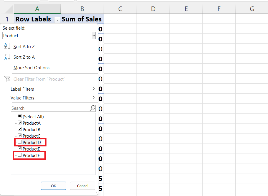
– Unselect the values you want to filter by unchecking the checkboxes right next to them.
Step 3 – Click on OK
– Click on OK in the drop-down menu.
– The selected values will be filtered from the pivot table


