
How to Drill Down into a pivot table
 By
SpreadCheaters
By
SpreadCheaters
Pivot Tables are a powerful tool in Excel that allows you to quickly and easily summarize large datasets. However, one of the useful features of PivotTables is the ability to Drill Down and explore the underlying data in more detail. Drill Down in pivot table refers to the ability to view and analyze the underlying data that makes up a summary value in the PivotTable. For example, if you have a PivotTable that shows the total sales by region, you are able to Drill Down on a specific region to see the individual sales transactions that make up the total sales figure. This allows you to analyze or investigate the data in more detail.
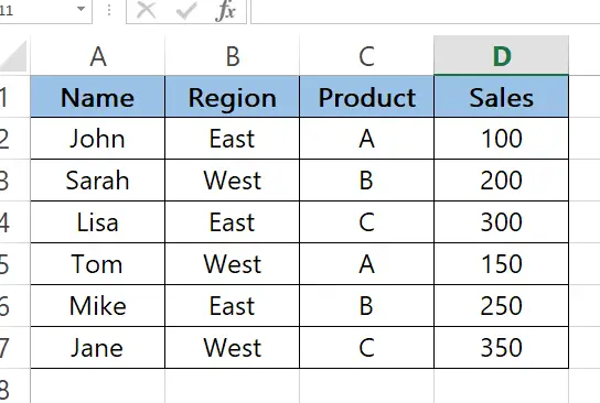
Here we have an example dataset that contains four columns which are Name, Region, Product, and Sales. In this tutorial, we will see how to Drill Down into the PivotTable by following the simple steps below. Let’s have a look at the dataset first.
Step – 1 Go to the Insert tab
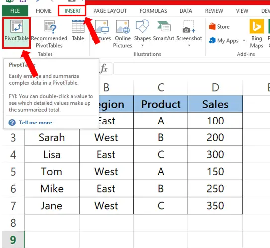
– First of all select the dataset.
– Click on the Insert tab.
– Go to the Tables group click on the PivotTable.
Step – 2 Create the PivotTable
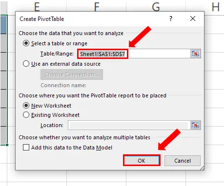
– After you have clicked on the PivotTable.
– Create PivotTable menu will appear.
– Range of the tale is selected already which is shown in Table/Range
– Check the options according to your needs.
– Click OK.
Step – 3 Add the data in the PivotTable
– In the PivotTable fields select the data you want in the PivotTable.
– In our case we selected Region, Product, and Sales.
– You can represent your pivot table according to your needs by dragging the fields into different categories. For example, e.g. in our case, we moved Region into Rows, Product into Columns, and Sales into Values to get the total sum of sales. For better understanding follow the video below.
Step – 4 Drill Down into the PivotTable

– To Drill Down, you can try double-clicking on a specific value in the PivotTable. For example, you could double-click on the value for East in the Region field to see the sales data for the East region. Similarly, you could double-click on the value for A in the Product field to see the sales data for product A.
– Another option is to right-click on a value and select Show Details to see the underlying data for that value in a new worksheet as shown below.


