How to do a multiplication formula in Google Sheets

In today’s tutorial, we will learn to perform multiplication in google sheets. In Google Sheets, multiplication is a mathematical operation that allows you to multiply two or more numbers together within a cell or range of cells. The overall importance of multiplication formulas in Google Sheets (and in spreadsheets in general) is that they allow you to automate calculations involving large amounts of data quickly and accurately.

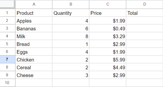
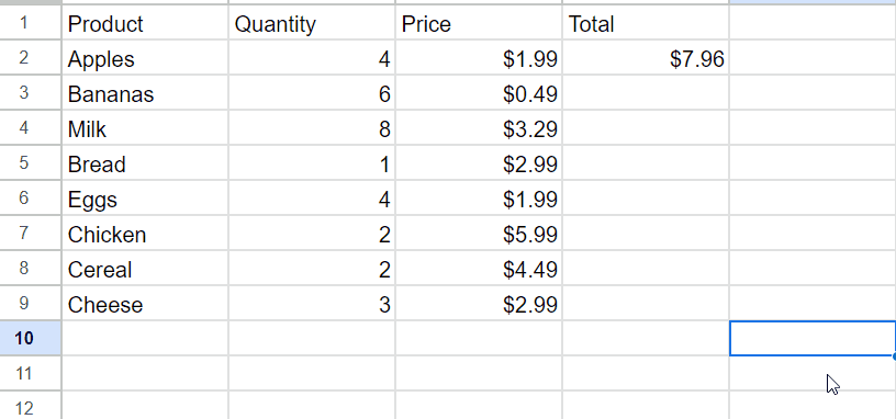
Our dataset is comprised of a grocery store bill that includes the names of the products, their corresponding quantities and prices, and the total amount. To calculate the total amount, we need to multiply the quantity by the price of each product. To perform this multiplication operation, we have four different methods at our disposal.

Method 1: Multiply using the Steric key(*)

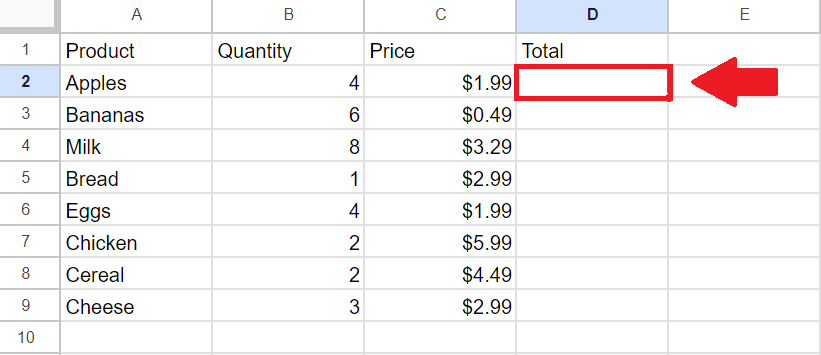
Step 1 – Select the Cell

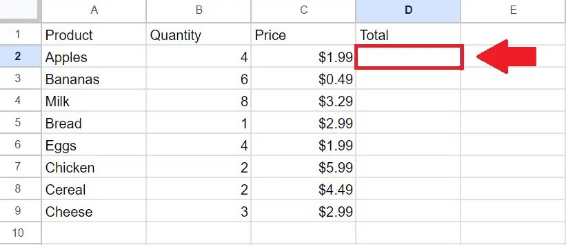
• Select the cell where you want to show the result of the multiplication

Step 2 – Type the Formula

• After selecting the cell, type the formula
• =Address of First Cell*Address of Second Cell
• Here it is =B2*C2

Step 3 – Press the Enter key

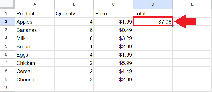
• After typing the formula, press the Enter key to get the result

Step 4 – Apply on Complete Column

• After getting the result in the first cell, move the cursor to the right bottom of the cell and a plus symbol will appear
• Click on this symbol and drag it to the desired cell of the column to get the required result

Method 2: Multiply using the Product function

Step 1 – Select the Cell

• Select the cell where you want to show the result of the multiplication

Step 2 – Use the Product function

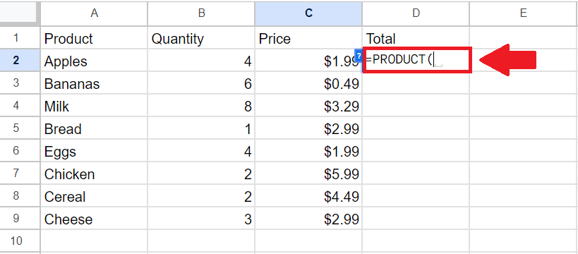
• After selecting the cell, type “=Product( ” to use the product function

Step 3 – Type the Arguments

• After typing the function, type its argument
• First Agument: Address of the first cell to multiply(Here it is B2)
• Second Argument: Address of the second cell to multiply(Here it is C2)

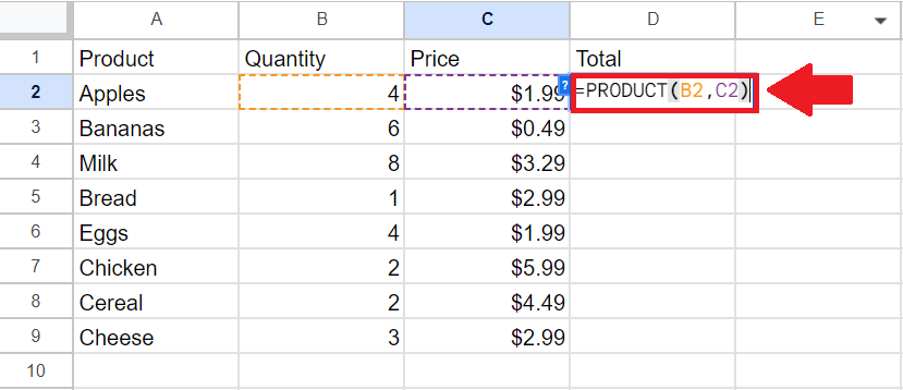
Step 4 –  Press the Enter key

• After typing the formula, press the Enter key to get the result

Step 5 – Apply on Complete Column

• After getting the result in the first cell, move the cursor to the right bottom of the cell and a plus symbol will appear
• Click on this symbol and drag it to the desired cell of the column to get the required result

Method 3: Multiply using the MULTIPLY function

Step 1 – Select the Cell

• Select the cell where you want to show the result of the multiplication

Step 2 – Use the Multiply function

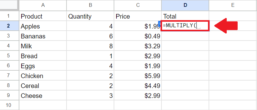
• After selecting the cell, type “=Multiply( ” to use the product function

Step 3 – Type the Arguments

• After typing the function, type its argument
• First Agument: Address of the first cell to multiply(Here it is B2)
• Second Argument: Address of the second cell to multiply(Here it is C2)

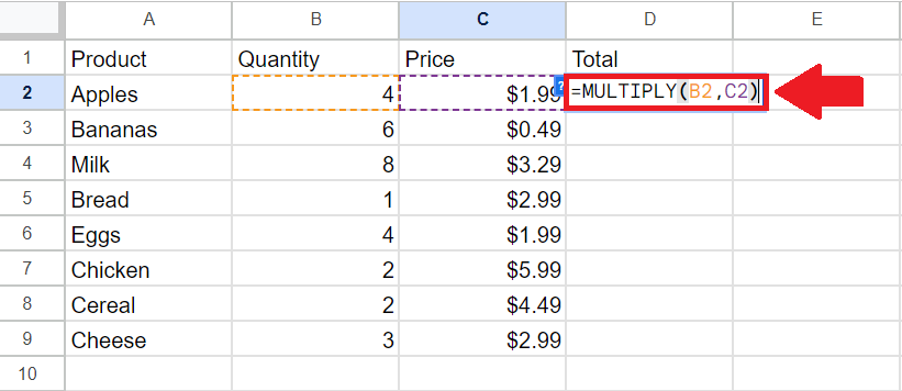
Step 4 –  Press the Enter key

• After typing the formula, press the Enter key to get the result

Step 5 – Apply on Complete Column

• After getting the result in the first cell, move the cursor to the right bottom of the cell and a plus symbol will appear
• Click on this symbol and drag it to the desired cell of the column to get the required result

Method 4: Multiply Two Columns

Step 1 – Select the Cell

• Select the cell where you want to show the result of the multiplication

Step 2 – Type the Formula

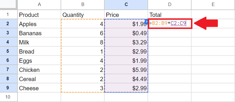
• After selecting the cell, type the formula
• =Range of First Cells*Range of Second Cells
• Here it is =B2:B9*C2:C9

Step 3 – Press the CTRL+Shift+Enter keys

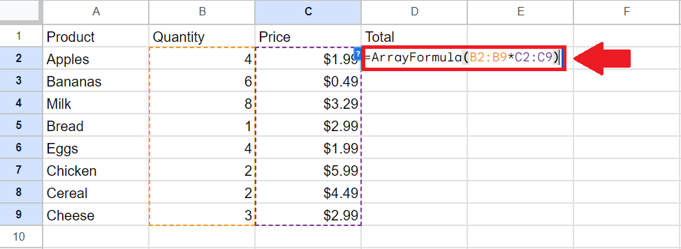
• After typing the formula, press the CTRL+Shift+Enter keys and the formula will be converted into an Array Formula

Step 4 – Press the Enter key

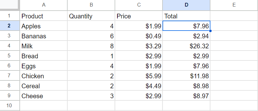
• After getting the ArrayFormula, press the Enter key to get the result