How to delete the last character in Excel 

 Deleting the last character in Excel refers to removing the rightmost character from a text string within a cell. The overall importance of deleting the last character in Excel lies in the ability to manipulate and modify textual data effectively. 

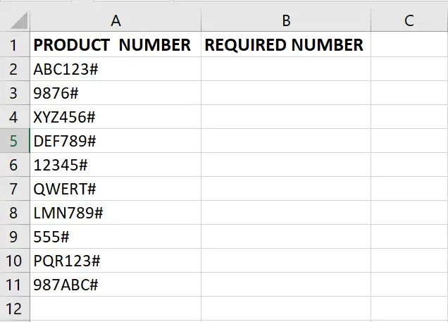
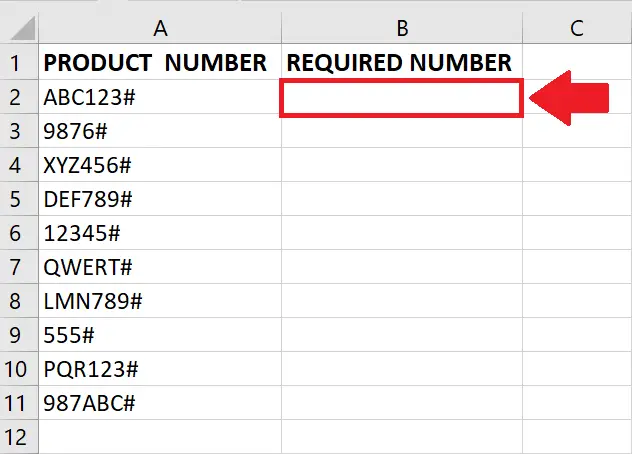
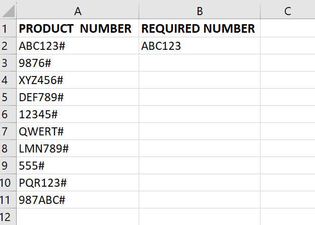
Our dataset has a list of product numbers, and each number ends with a hashtag. Our objective is to delete this last character from each number. To achieve this we have two methods that are explained below.  

Method 1: Delete the Last Character using the Replace option 

Step 1 – Select the Cell 

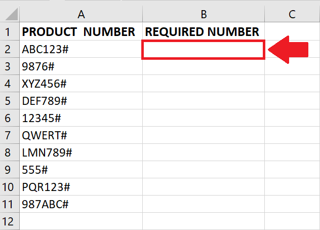
• Click on the cell where you want to show the result 

Step 2 – Use the Replace function 

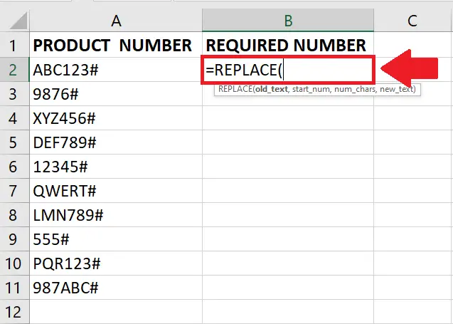
• After selecting the cell, use the Replace function by typing: 
• =REPALACE( 

Step 3 – Type the Argument 

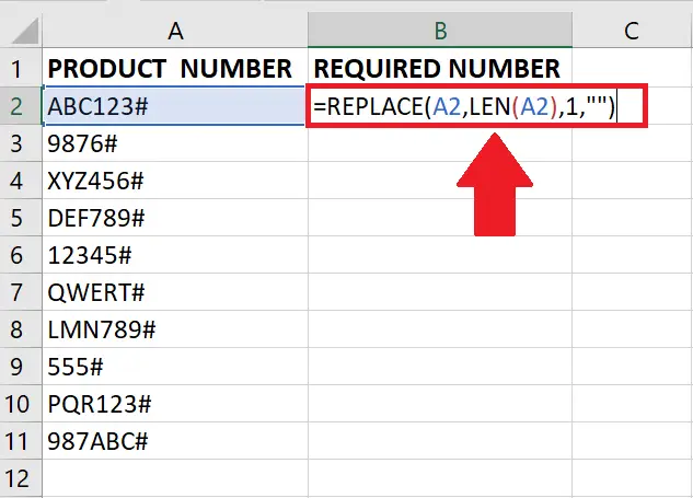
• Afterward, type the arguments of REPLACE  function as follow: 
• =REPLACE(A2,LEN(A2),1,””) 

A2: This refers to the cell containing the text string you want to modify. 

LEN(A2): The LEN function is used to calculate the length of the text string in cell A2. It determines the position of the last character in the string. 

1: This specifies the number of characters you want to replace. In this case, it is set to 1, indicating that we want to replace the last character only. 

“”: The empty quotation marks denote that we want to replace the last character with nothing, effectively deleting it. 

Step 4 – Press the Enter key 

• Press the ENTER key after typing the arguments to get the result in the cell 

Step 5 – Copy the Function in Column 

• After getting the result in the cell, drag the cell down in the column till the required cell 

Method 2: Delete the Last Character using the LEFT function 

Step 1 – Select the Cell 

• Click on the cell where you want to show the result 

Step 2 – Use the TRIM function 

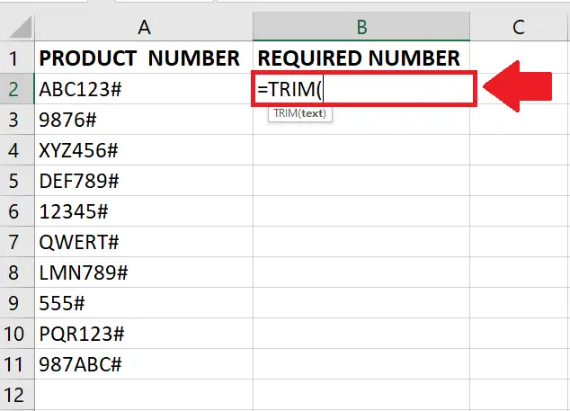
• After selecting the cell, use the TRIM  function by typing: 
• =TRIM( 

Step 3 – Type the Argument 

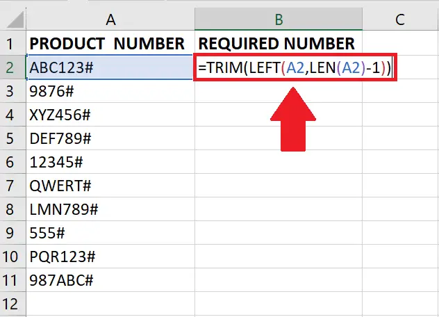
• Afterward, type the arguments of the TRIM function as follow: 

• =TRIM(LEFT(A2,LEN(A2)-1)) 

A2: This refers to the cell containing the text string you want to modify. 

LEN(A2): The LEN function calculates the length of the text string in cell A2, giving the total number of characters. 

LEN(A2)-1: Subtracts 1 from the length to exclude the last character. 

LEFT(A2, LEN(A2)-1): The LEFT function takes the leftmost characters from cell A2, excluding the last character based on the calculated length. 

TRIM(LEFT(A2, LEN(A2)-1)): The TRIM function deletes any leading or trailing spaces from the result. 

Step 4 – Press the Enter key 

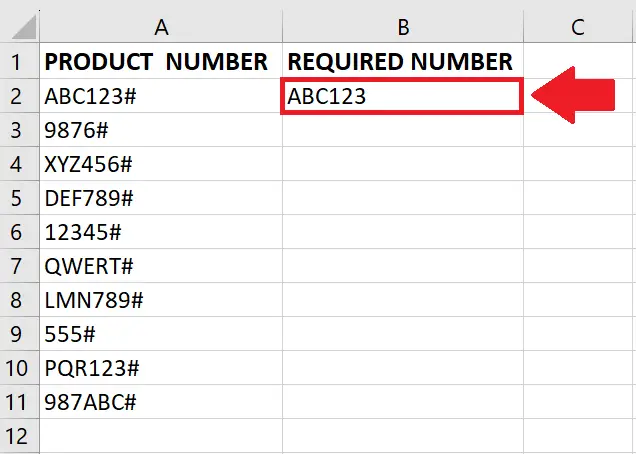
• Press the ENTER key after typing the arguments to get the result in the cell 

Step 5 – Copy the Function in Column 

• After getting the result in the cell, drag the cell down in the column till the required cell