How to remove first character in Excel

Excel is a very powerful tool to perform mathematical and statistical calculations on numeric data. However, it provides a variety of tools and functions to handle and manipulate text and alphanumeric data as well. Sometimes, when you receive data from someone else or from web sources, there are unwanted characters just before the start of data in each cell. 

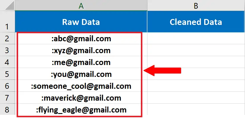
Let’s take a look at the following dataset which has the : symbol added before each email address. In this tutorial, we’ll learn how to use the below mentioned methods to replace the first unwanted character from the data.

• Flash Fill
• Replace function
• Right function
• Find and Replace Tool

All methods are very simple to use and let’s explore each of them by following the steps mentioned in the sections below.

Method 1: Use Flash Fill

This is the easiest of all methods to be used for this purpose. This can be used to replace the first character by creating a .

Step 1 – Create a sample data point with clean data

• To use the Flash fill feature of Excel, we need to create a sample data point for Excel to follow the pattern. So write the desired email address without the : colon sign,  right in the cell next to the raw data as shown below.

abc@gmail.com

• Now we’ll use the Flash Fill too by pressing CTRL+E, this will clean the whole data by removing the first unwanted character i.e., : colon sign from the data.

Method 2: Use REPLACE function

The syntax of this function is very simple as shown below,

REPLACE(old_text, start_num, num_chars, new_text)

The REPLACE function has the following arguments:

• Old_text    

Text in which you want to replace some characters.

• Start_num    

The position of the character in old_text that you want to replace with new_text. We’ll use 1 because we want to remove the first character.

• Num_chars    

The number of characters in old_text that you want REPLACE to replace with new_text. We’ll again use 1 as we wish to remove only the first character.

• New_text  

The text that will replace characters in old_text. We’ll replace the first character by a void string using “” characters.

Step 1 – Create the appropriate formula using REPLACE

• We can use the REPLACE function to remove the first character from the text very easily. This function is pretty straightforward to use, therefore, the following formula can be used to remove the first character from the data contained in cell A2.

=REPLACE(A2,1,1,””)

• This formula can be extended to the whole dataset by double clicking the fill handle as shown above.

Method 3: Use RIGHT function

The syntax of this function is very simple as shown below,

RIGHT(text, [num_chars])

The RIGHT function has the following arguments:

• Text    

This is the text string that contains the characters you want to extract. In our case, we wish to extract all characters except the first one.

• [num_chars]

This is an optional argument. It specifies the number of characters you want RIGHT to extract, counting from the right side of the text string. So, in our case, we’ll use a number which will be 1 less than the total length of the string, because we wish to extract all characters except the first one. So, we’ll use LEN(A2) -1 to get the number 1 less than the length of the string.

• num_chars must be greater than or equal to zero.
• If num_chars is greater than the length of text, RIGHT returns all of the text.
• If num_chars is omitted, it is assumed to be 1.

Step 1 – Create the appropriate formula using RIGHT

• We can use the RIGHT function to remove the first character from the text very easily. We’ll use the following formula to remove the first character from the data contained in cell A2. We used LEN(A2) -1 to get the number 1 less than the length of the string and this will return all characters except the first one.

=RIGHT(A2, LEN(A2)-1)

• This formula can be extended to the whole dataset by double clicking the fill handle as shown above.

Method 4: Use Find & Replace Tool

If you don’t like to use formulas and want to clean the data by keeping it in its original place then you should use the Find and Replace tool. However, this will change your source data as well. All above methods didn’t change the source data, rather we created another column for the cleaned data.

Step 1 – Use CTRL + H to open up Find & Replace Tool

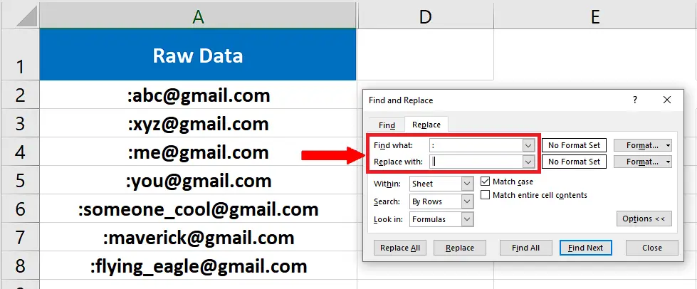
• Press CTRL + H to open up the Find & Replace tool.
• Write : in Find what and blank space in Replace with as shown above.

Step 2 – Use Replace All to clean data

• Press Replace All button to clean the data. It will automatically replace all instances of : colon sign from the source data.