How to create multiple PivotTables from one data source
This PivotTable summarizes the sales data for three products (Product A, Product B, and Product C) across four quarters (Q1, Q2, Q3, and Q4). The “Sum of Sales” column displays the total sales figures for each product and quarter combination, as well as the grand total for all products. We want to create two PivotTable from a single data source where one PivotTable will contain sales data from the first two quarters and the other will contain sales data from the last two quarters.
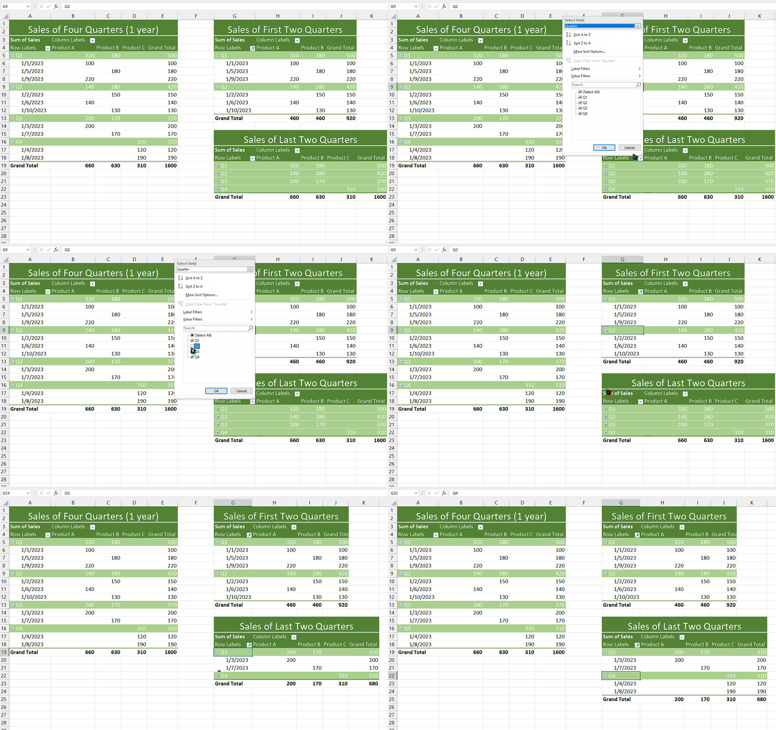
With multiple PivotTables, you can segment and filter your data in various ways. Each PivotTable can have its own set of filters, enabling you to focus on specific subsets of data or apply different criteria to analyze different aspects of your dataset.
Step 1 – Copy the PivotTable
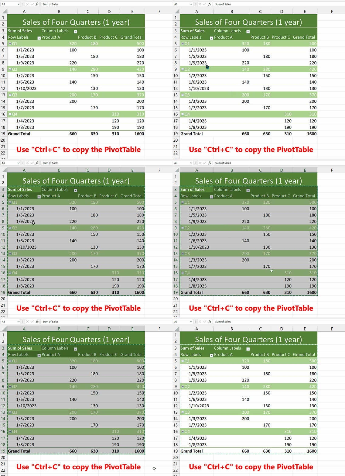
– Select the Pivot Table that encompasses the complete dataset from the source data.
– Press “Ctrl+C” to copy it.
Step 2 – Paste the Pivot Table in two separate locations
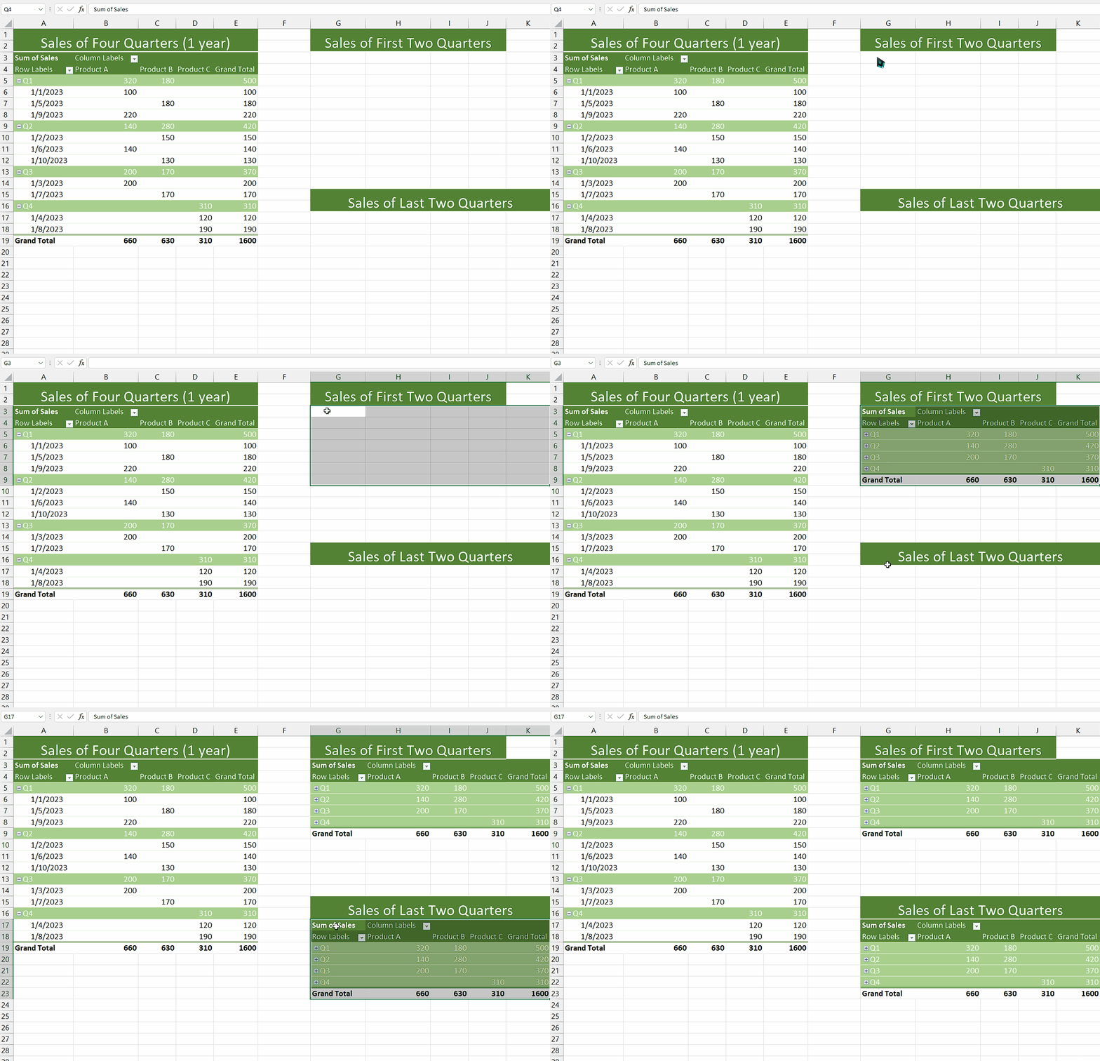
– After copying the PivotTable, paste it anywhere in the sheet you like.
– Then, paste the PivotTable again in some different area.
Step 3 – Filter the data from the first PivotTable
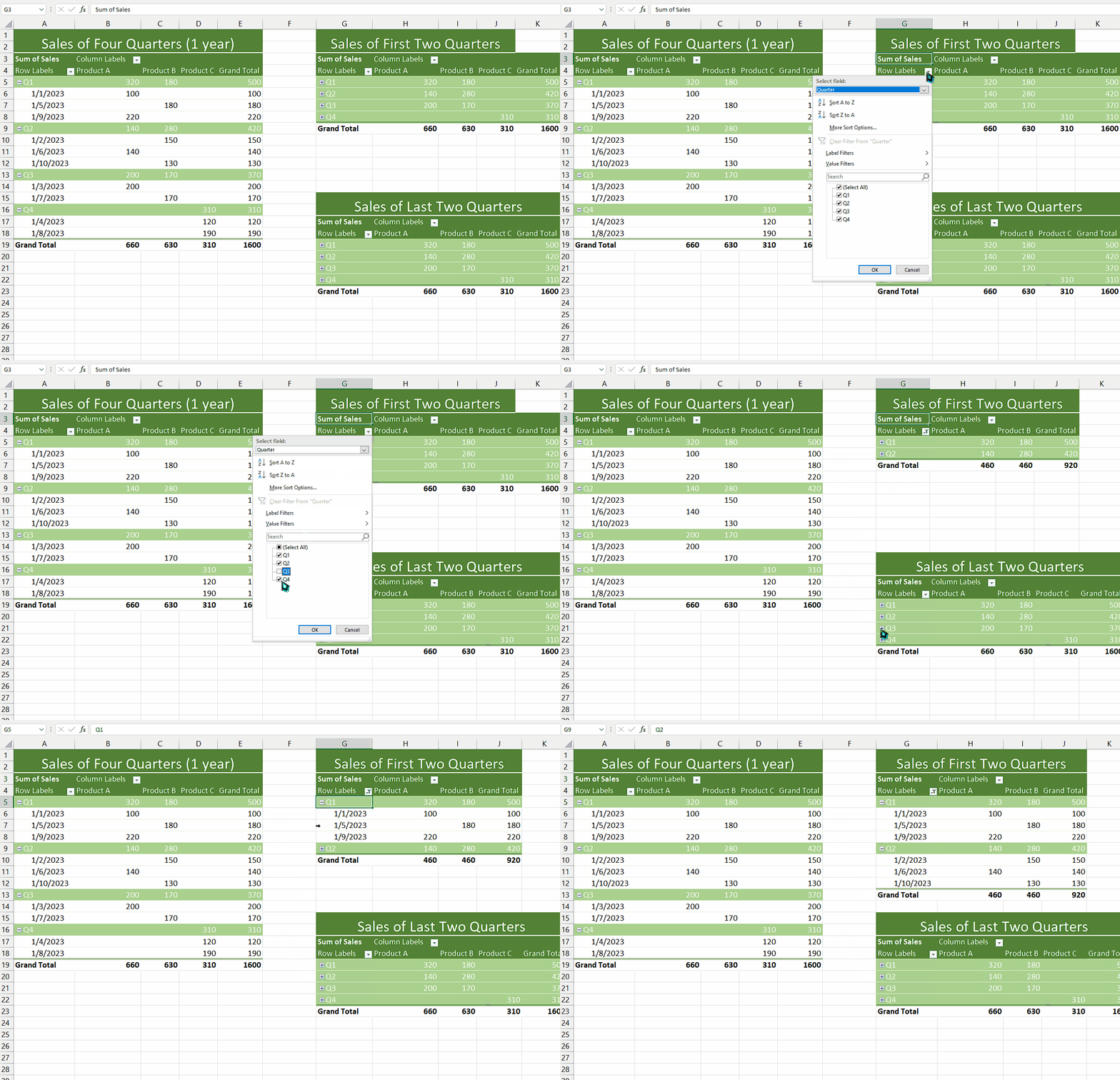
– First of all, make sure that your field headers of PivotTable are enabled.
– Then, choose the PivotTable from which you want to filter data first.
– If you want to filter data present in rows then click on the downward arrow in “Row Labels”.
– If you want to filter data present in columns then click on the downward arrow in “Column Labels”.
– Then, uncheck the rows or columns that you don’t want to include and check the rows or columns that you want to include.
– Now, your data from the First PivotTable will be filtered.
– For instance, we have excluded Q3 and Q4 from the PivotTable so it only contains sales data for the first two quarters.
Step 4 – Filter the data from the second PivotTable

– To begin, ensure that the field headers of your Pivot table are enabled.
– If you intend to filter data in the rows, click the downward arrow in the “Row Labels” section.
– If you want to filter data in the columns, click the downward arrow in the “Column Labels” section.
– Proceed by unchecking the rows or columns that you want to exclude, and checking the ones you want to include.
– The data in the second PivotTable will now be filtered accordingly.
– As an example, we have excluded Q1 and Q2 from this Pivot table so it only contains sales data for the last two quarters.


