
How to create a title row in Google Sheets
 By
SpreadCheaters
By
SpreadCheaters
In this tutorial, we will learn how to create a title row in Google Excel. The title plays a vital role in the visual appearance of the data. It can be created by adding a blank row above the data. The header can be formatted to make it visually appealing. The header row can be frozen so that the title row does not disappear when we scroll down.

In Google Sheets, a title row is the first row of a spreadsheet that contains the headers or titles for each column of data in the sheet. The title row is used to provide a clear and concise description of the data in each column and helps to organize the data in the sheet. The title row is usually formatted differently from the rest of the rows in the sheet to make it stand out, such as in bold or in a different font.
Step 1 – Right-Click on the Header of the First Row
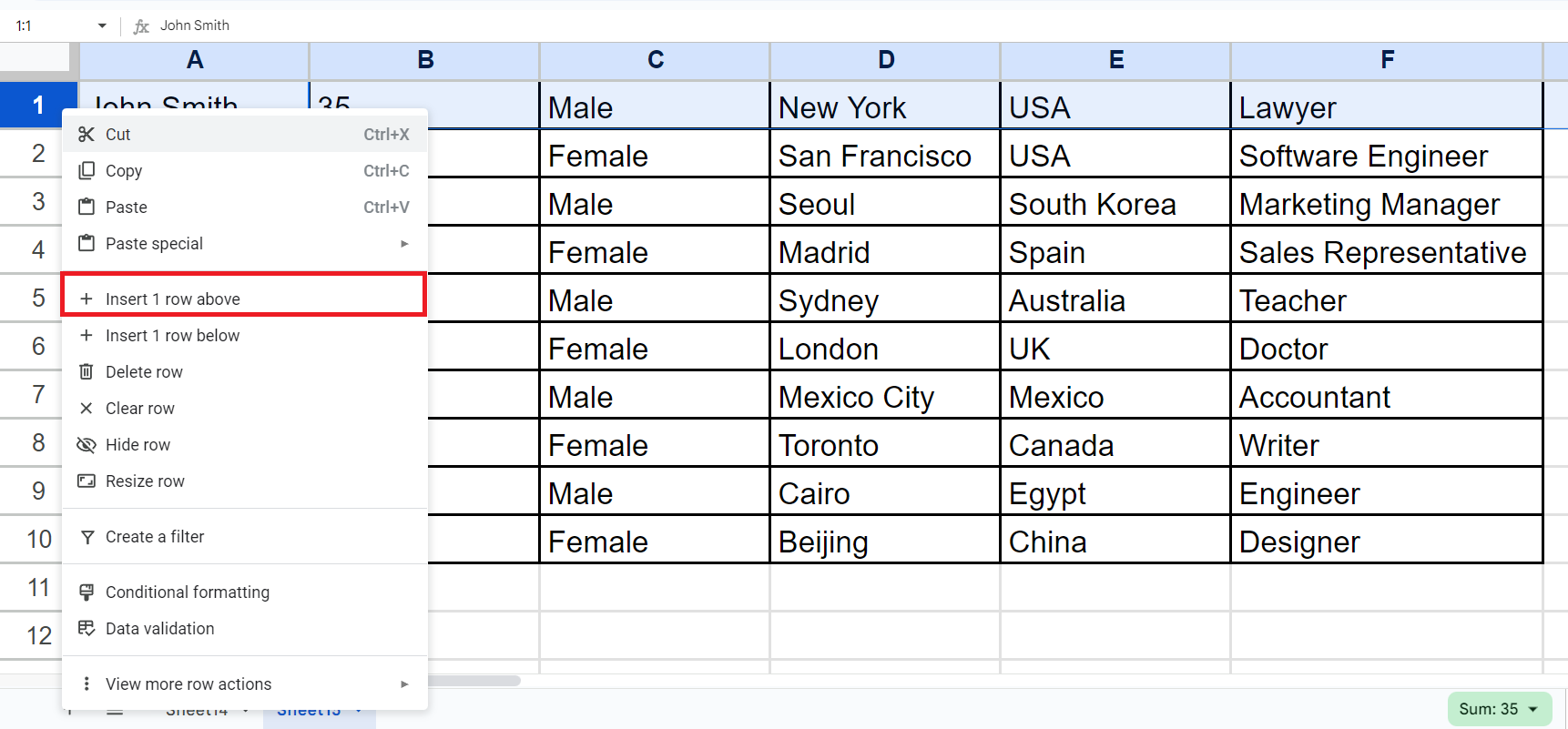
– Right-click on the header of the first row of the data.
– A context menu will appear.
Step 2 – Click on the “+ Insert 1 row above” Option
– Click on the “+ Insert 1 row above” option in the context menu.
– A blank row will be added above the data.
Step 3 – Add the Headers of Each Column
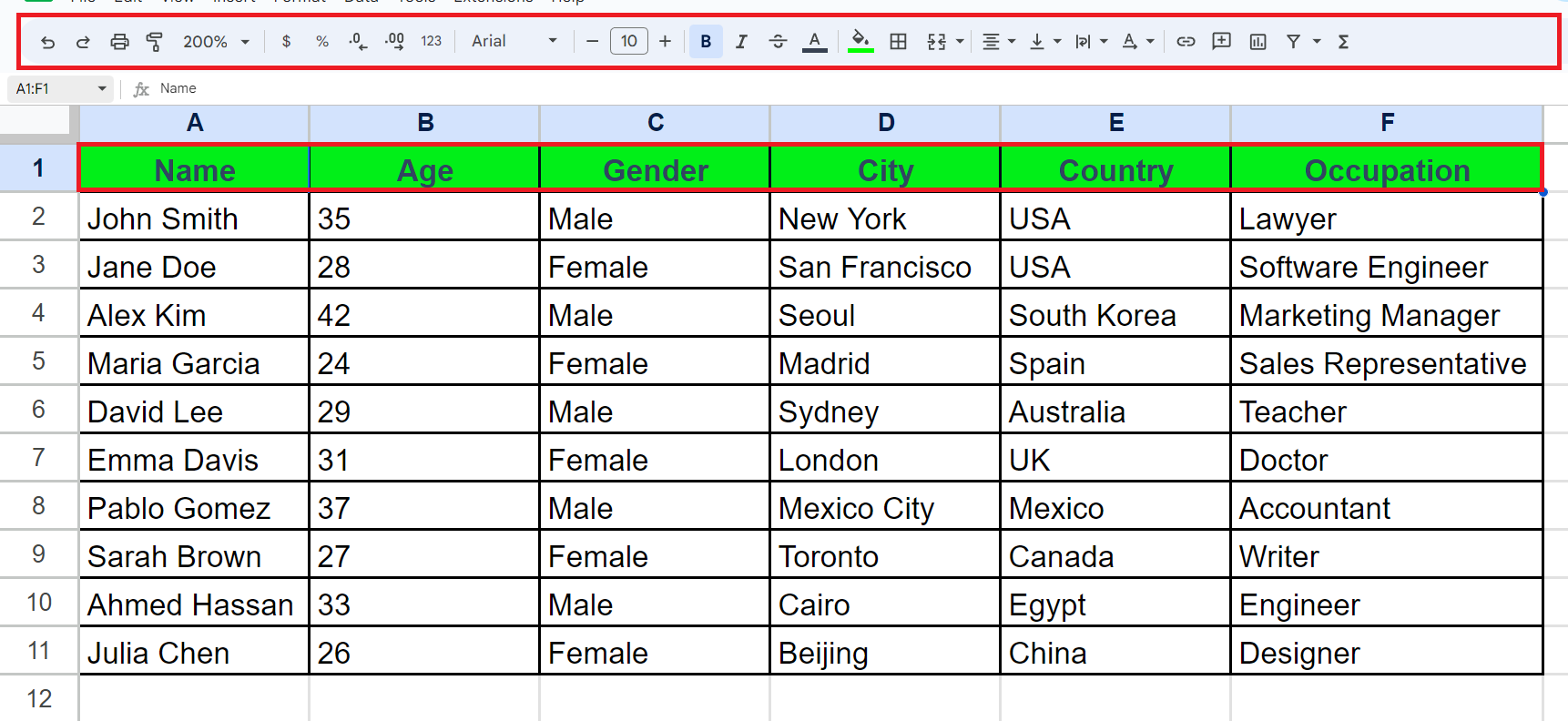
– Add the headers of each column in the blank row.
– You may format the headers using the options in the toolbar to make the Title Row visually appealing.
– The title row will be created.
Step 4 – Freeze the Title Row
– Freeze the Title row.
– For this, Select the row by clicking on the row header i.e. the row number on the left of the row.
– Click on the View menu and click on the Freeze option.
– Select “Upto row 1”, where 1 is the number of the Title Row.
– The Title row will be frozen.
Step 5 – Scroll Down to Check If the Title Row is Frozen
– Scroll down in the sheet to check if the Title row is always visible.


