How to count a list of names in Excel 

To count a list of names in Excel means to determine the total number of occurrences of specific names within a given range of cells. Overall, counting a list of names in Excel provides valuable insights and facilitates data analysis, validation, reporting, and data management tasks.  

In this tutorial, we will learn how to count a list of names in Excel. We have three methods available below to count the names in our dataset, which consists of a list of people participating in a lucky draw. 

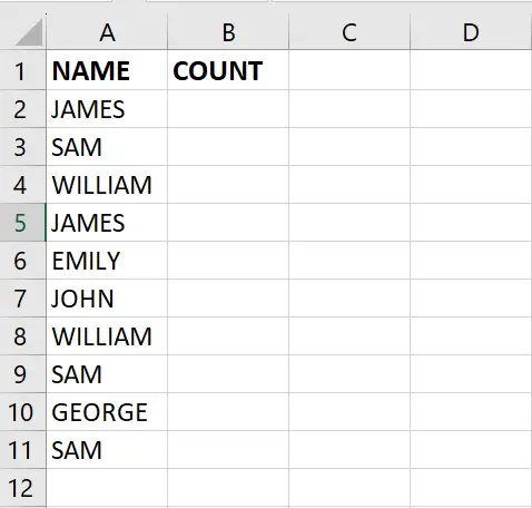
Method 1: Count the Total Number of Names 

Step 1 – Select the Cell 

• Click on the cell where you want to show the result 

Step 2 – Use the COUNTA function 

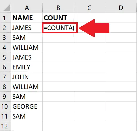
• After selecting the cell, use the COUNTA function 

Step 3 – Type the Argument  

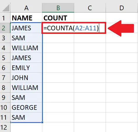
• After using the function, type the arguments 
• After typing the arguments, place an ending bracket 
• =COUNTA(A2:A11) 

Step 4 – Press the Enter key 

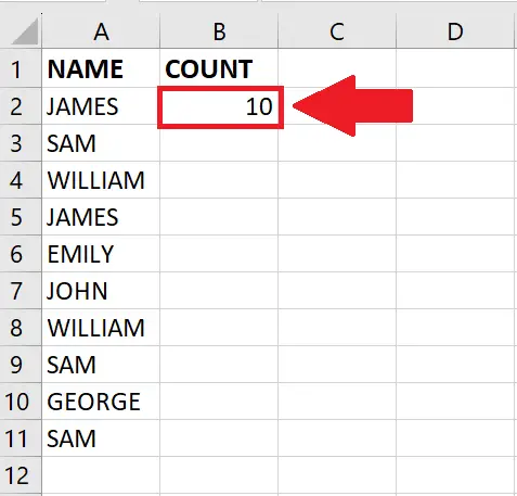
• Afterward, press the Enter key to get the result 

Method 2: Count the Total Number of occurrences of a specific Name in the list using the SUMPRODUCT function 

Step 1 – Select the Cell 

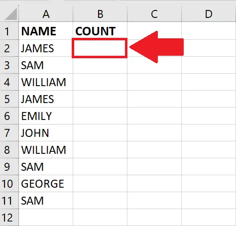
• Click on the cell where you want to show the result 

Step 2 – Type the Formula 

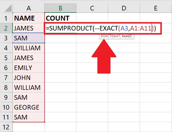
• After selecting the cell, type the following formula: 

=SUMPRODUCT(–EXACT(A3,A1:A11)) 

EXACT(A3, A1:A11): This part compares each cell in the range A1:A11 with the value in cell A3 and returns an array of TRUE or FALSE values. TRUE indicates an exact match, and FALSE indicates a mismatch. 

–EXACT(A3, A1:A11): The double unary operator “–” is used to convert the TRUE and FALSE values to 1s and 0s, respectively. This is necessary because SUMPRODUCT expects numeric values. 

SUMPRODUCT(–EXACT(A3, A1:A11)): Finally, the SUMPRODUCT function multiplies each element of the converted array by 1 (if it’s a match) or 0 (if it’s not a match) and then sums up the resulting array. The result is the count of cells that match the value in A3. 

Step 3 – Press the Enter key 

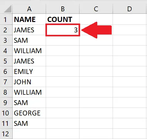
• Afterward, press the Enter key to get the result 

Method 3: Count the Total Number of occurrences of a specific Name in the list using the CountIF function 

Step 1 – Select the Cell 

• Click on the cell where you want to show the result 

Step 2 – Type the Formula 

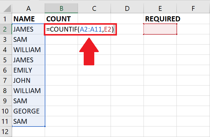
• After selecting the cell, type the following formula: 
• =COUNTIF(A2:A11,E2) 
• “COUNTIF” is a function used to count the number of cells in a range that meet a specific condition. 
• “A2:A11” refers to the range of cells from A2 to A11, where the function will check for matches. 

• “E2” is the criteria or value that the function will use to determine if a cell in the range matches the criteria. 
•  

Step 3 – Get the Result 

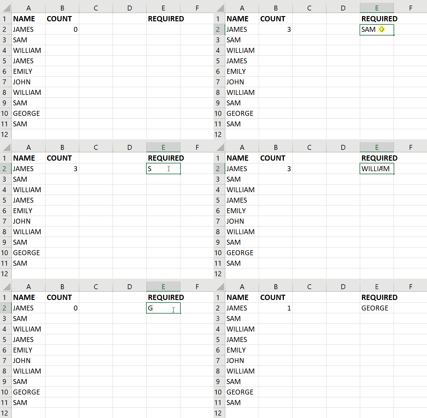
• After typing the formula, click on the Criteria cell and type the name whose occurrence is required 
• Then press the Enter key to get the required result