
How to create a tier list in Microsoft Excel
 By
SpreadCheaters
By
SpreadCheaters
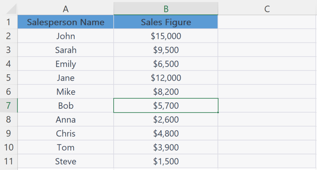
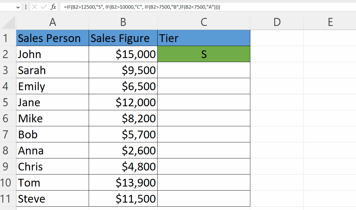
In this tutorial, we will learn how to create a tier list in Microsoft Excel. With the help of Excel’s pre-installed features and functions, generating a tier list that is both visually appealing and user-friendly can be accomplished with ease. We have a data set above that shows the sales figures of different salespeople, and we wish to categorize these figures into different tiers based on specific values. Specifically, we want to create a tier list and assign each sale figure a corresponding tier label. The tiers we want to use are S (for sales figures above $12500), C (for sales figures above $10000), B (for sales figures above $7500), and A (for sales figures below $7500).
Creating a tier list in Excel means sorting and classifying items according to particular criteria and allotting each item to a particular tier based on its perceived level of importance or quality. A tier list usually comprises several tiers, each representing a different ranking or priority level.
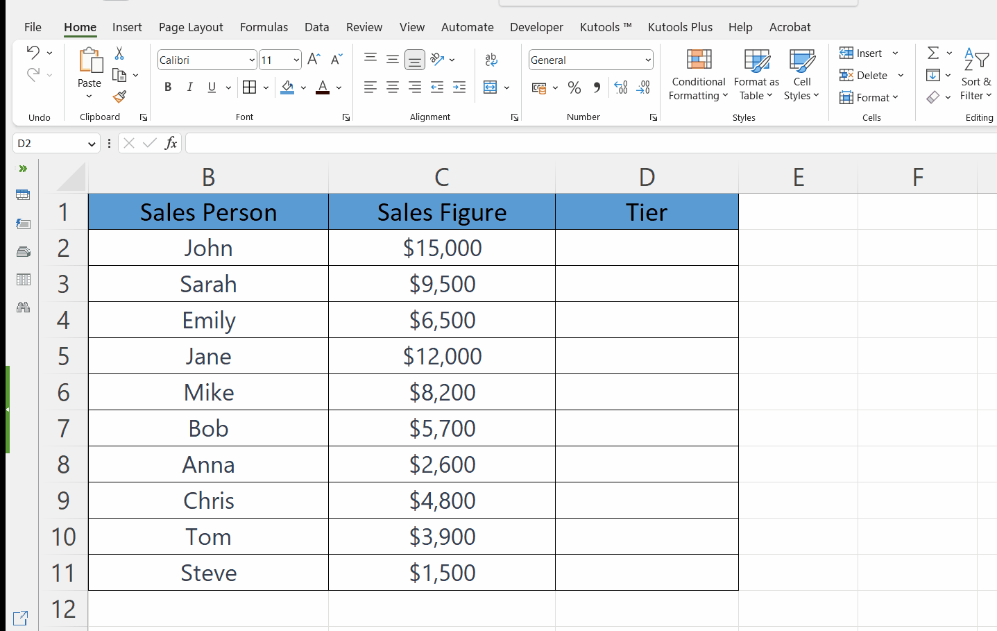
Step 1 – Set a New Spread Sheet for a Tier List
– Set up a new spreadsheet for a tier list.
Step 2 – Assign the Name of Salespersons to the First Column
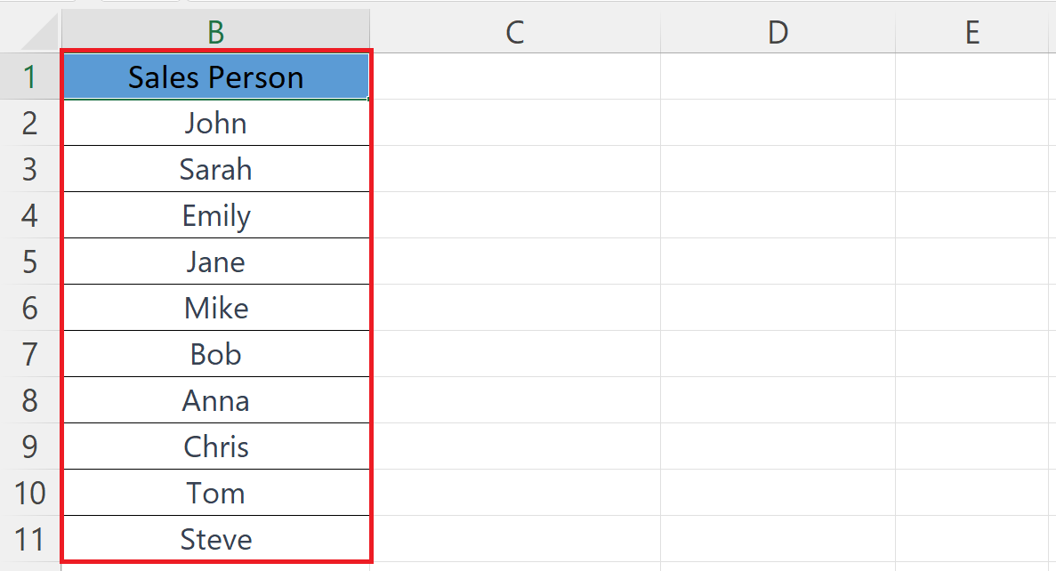
– Assign the names of salespersons to the first column.
Step 3 – Input the Sales Figures in the Second Column
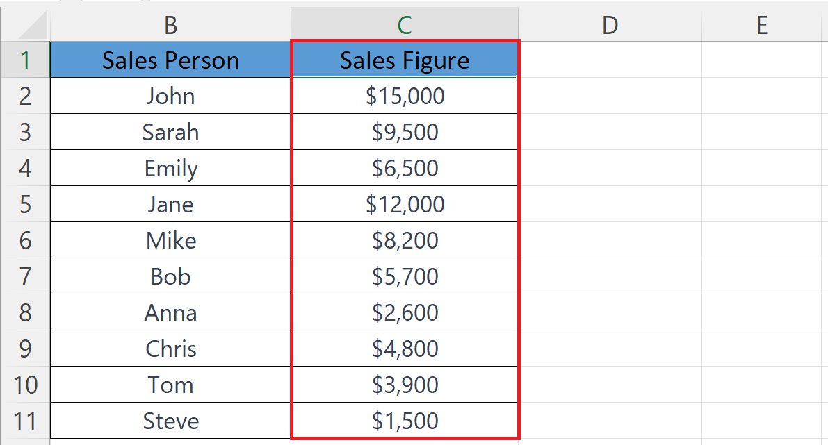
– Input the sales figures in the second column.
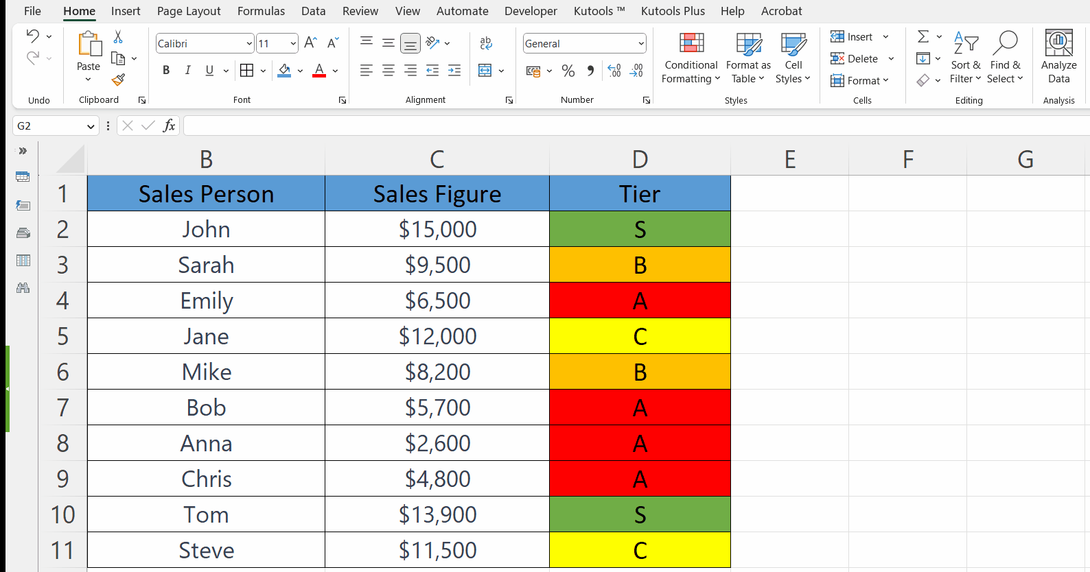
Step 4 – Set the Third Column for Tier
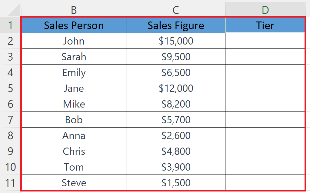
– Set the third column for tiers i.e. A, B, C, S.
Step 5 – Apply Conditional Formatting to the Tier Column
– Apply Conditional formatting to the column with tiers.
– Here we have assigned “Green” color for the cells containing “S”, “Yellow” for “C”, “Orange” for “B” and “Red” for “A”.
– To set specific colors we can utilize the custom format option after setting the rule i.e. “cell that contains” or “Equal to”.
Step 6 – Assign Tiers to the First Salesperson Utilizing the IF Function
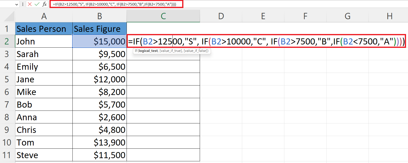
– Assign tiers to each salesperson in the Tier column utilizing the IF function.
– The structure of the IF function, in this case, would be:
=IF(B2>12500,”S”, IF(B2>10000,”C”, IF(B2>7500,”B”,IF(B2<7500,”A”))))
– There are three nested IF functions in the Parent IF function.
– The initial IF statement evaluates if a value exceeds $12500, if yes, then it outputs “S”.
– If the first statement is false, the second IF statement is evaluated to check if the value exceeds $10000, and if yes, then it outputs “C”.
– If the second statement is also false, the third IF statement is evaluated to check if the value exceeds $7500, and if yes, then it outputs “B”.
– If all three statements are false, the fourth and final IF statement evaluates if the value is less than or equal to $7500 and if yes, then it outputs “A”.
Step 7 – Assign Tiers to Each Salesperson Utilizing the IF Function
– Assign Tiers to each salesperson using Autofill.
Step 8 – Sort the Tier Column

– Sort the Tier column using the option “Sort Z to A”, located in the Editing section of the Home tab.
– Choose the “Expand the Selection” option in the dialog that appears.


