How to copy filtered data in Excel to another sheet 

Copying filtered data from one sheet to another in Excel is a valuable practice with several benefits. By doing so, we can segregate and organize data based on specific criteria, allowing for more focused analysis and streamlined workflow. By separating the filtered data, we can perform further analysis without altering the original dataset. This approach enhances data security, reduces the risk of errors, and facilitates efficient decision-making. 

The dataset given below contains sales transaction information, including a unique order ID, customer names, purchased products, purchase dates, and addresses. It can be used to analyze sales performance, trends, customer demographics, and geographical distribution of sales, aiding in market analysis and informed decision-making. We will use this dataset to learn how to Filter the data and then copy it to another sheet. 

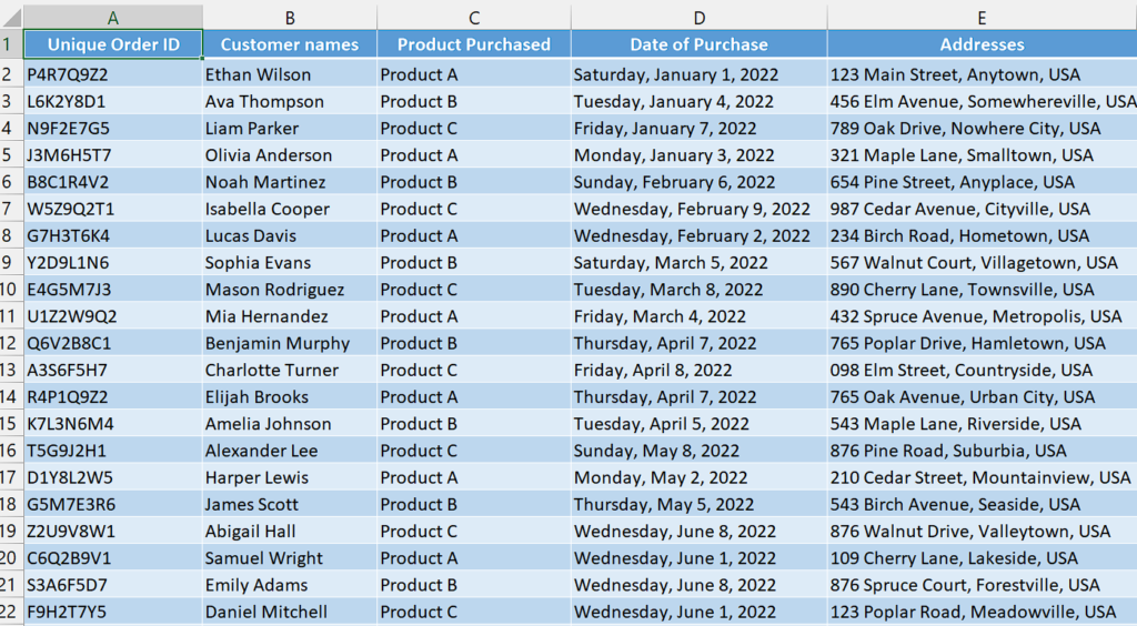
Method 1 – By manually copying and pasting 

Step 1 – Create filters 

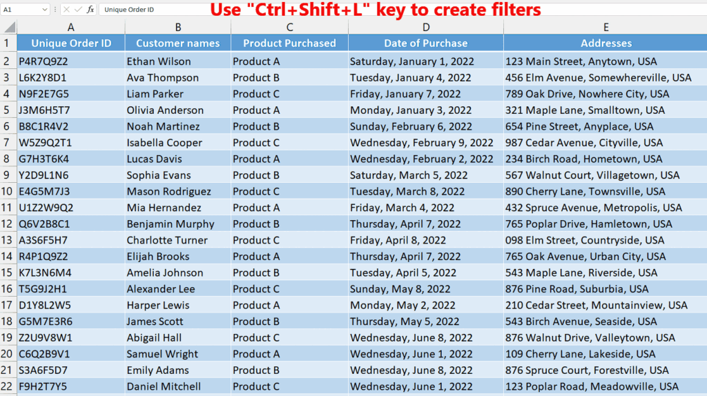
• Select any cell of your dataset. 
• Then, use the “Ctrl+Shift+L” key to create filters. 

Step 2 – Filter Desired Data 

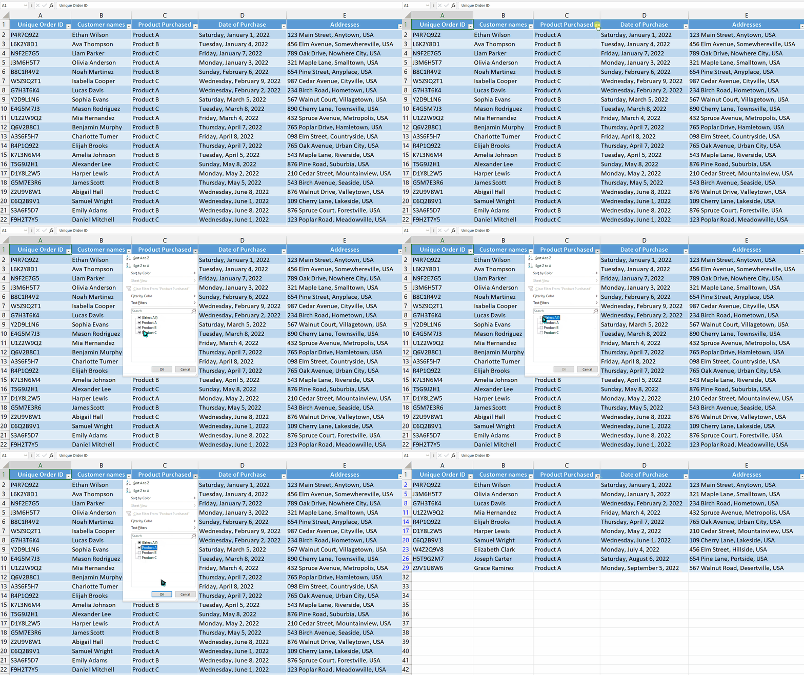
• To begin filtering the data, click on the downward arrows in the cell headers to reveal a drop-down list.  
• From there, select the desired data to filter. For instance, if you want to view only sales of Product A, simply check the box corresponding to Product A and uncheck all other boxes. 

Step 3 – Copy the Data 

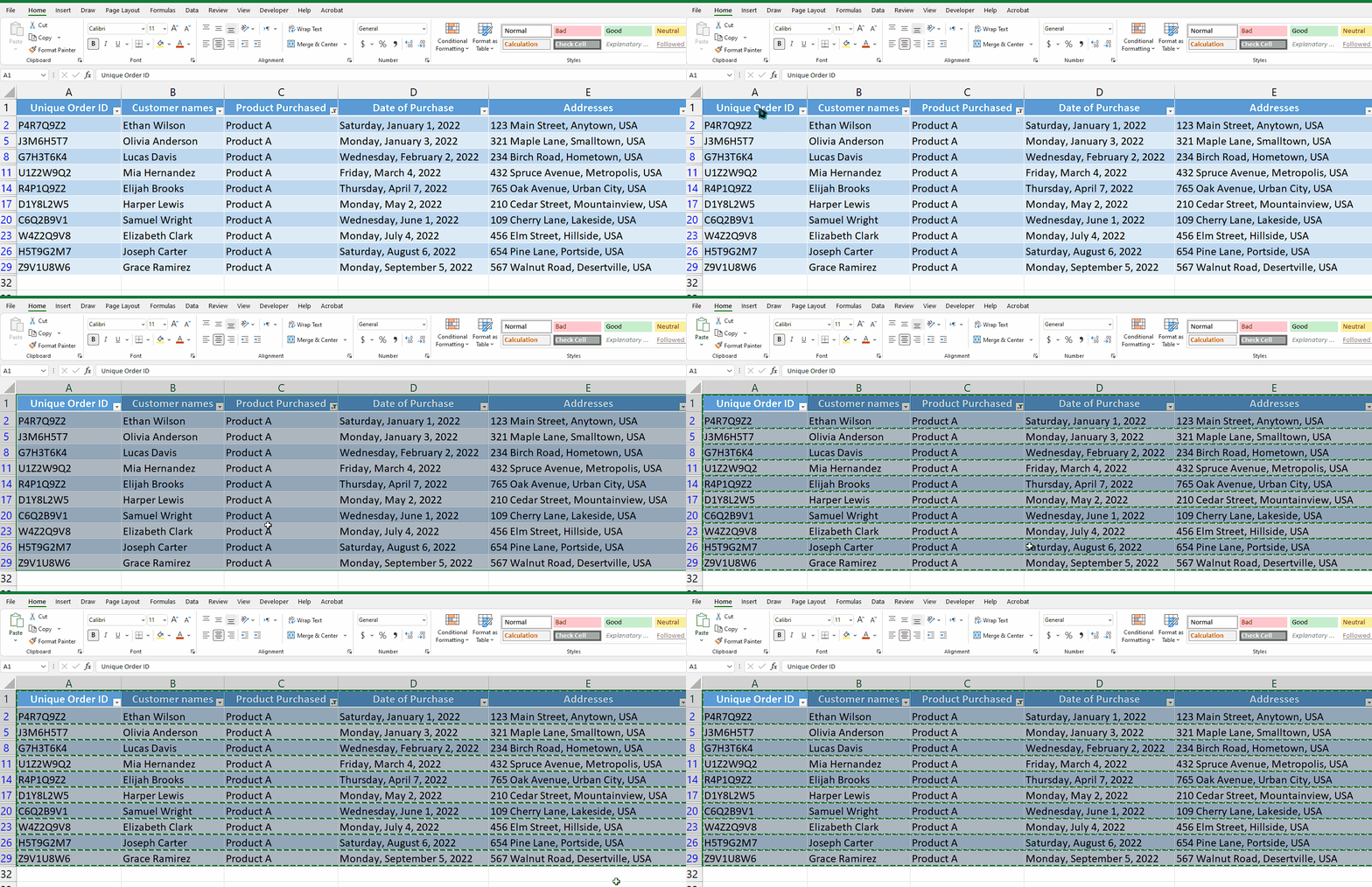
• Now, select the whole filtered data and then use the “Ctrl+C” key to copy the data. 

Step 4 – Paste on the required sheet 

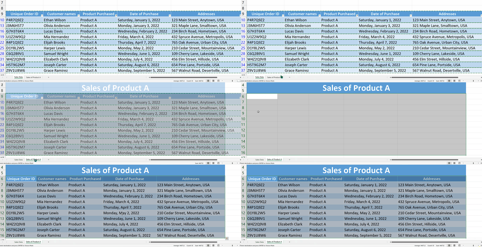
• Proceed by clicking on the tab of the second sheet to access the desired destination where you intend to paste the filtered data. 
• Next, select the cell where you want to paste the filtered data. Keep in mind that this cell will serve as the starting point for the filtered data, and the remaining data will follow the pattern accordingly. 
• Now, use “Ctrl+V” to paste the data. 

Method 2 – By using the VBA code 

Step 1 – Insert a module 

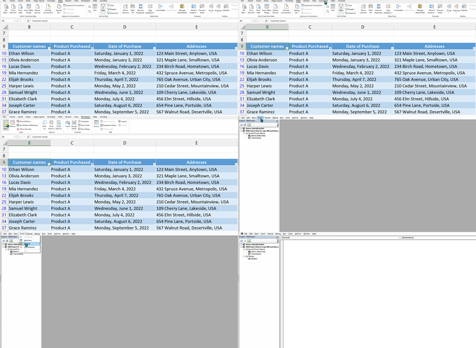
• For adding a module, navigate to the Developer tab. 
• After that, click on the first option named Visual Basic. 
• You’ll see a new window on your screen and you can also open this window by using the shortcut key (Alt+F11) as well. 
• Then, click on the Insert tab in this window and click on the Module option. 

• Now, a new module would open. 

Step 2 – Write the code 

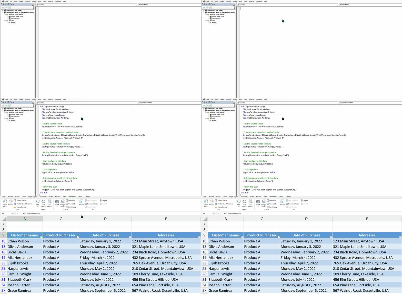
• Copy and paste the following code in the module and make the necessary changes to select the range of filtered data and change the name of the newly created sheet. 

Sub CopyAndPasteData() 
Dim wsSource As Worksheet 
Dim wsDestination As Worksheet 
Dim rngSource As Range 
Dim rngDestination As Range 
 
‘ Set the source sheet 
Set wsSource = ThisWorkbook.ActiveSheet 
 
‘ Create a new sheet for the destination 
Set wsDestination = ThisWorkbook.Sheets.Add(After:=ThisWorkbook.Sheets(ThisWorkbook.Sheets.Count)) 
wsDestination.Name = “Sales of Product A” 
 
‘ Set the source range to copy 
Set rngSource = wsSource.Range(“A9:E37”) 
 
‘ Set the destination range to paste 
Set rngDestination = wsDestination.Range(“A1”) 
 
‘ Copy and paste the data 
rngSource.Copy rngDestination 
 
‘ Clear clipboard 
    Application.CutCopyMode = False 
 
‘ Adjust column widths to fit the data 
    wsDestination.Columns.AutoFit 
 
‘ Notify the user 
MsgBox “Data has been copied and pasted successfully.” 
End Sub 

• Then, close the VBA Editor. 

Step 3 – Run the macro 

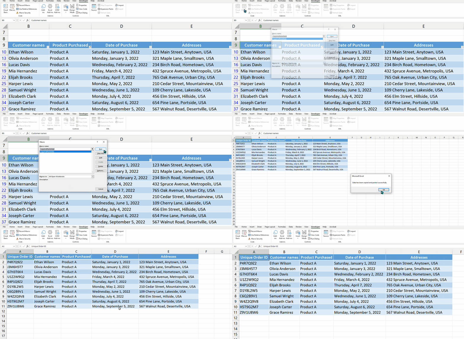
• Click on the “Developer” tab in the Excel ribbon. If you don’t see the “Developer” tab, you may need to enable it. Go to the Excel options and enable the “Developer” tab. 
• In the “Developer” tab, click on the “Macros” button. This will open the “Macro” dialog box. 

• In the “Macro” dialog box, you should see a list of available macros in your workbook. Select the “CopyAndPasteData” macro from the list. 
• Click on the “Run” button. This will execute the selected macro. 
• The macro will perform its assigned tasks, such as copying and pasting data according to its programmed instructions. 

Explanation of code used in Method 2: 

This VBA code copies data from the active sheet in an Excel workbook to a newly created sheet named “Sales of Product A”. The data is copied from cells A9 to E37 on the source sheet and pasted starting from cell A1 on the destination sheet. The column widths in the destination sheet are adjusted to fit the data, and a message box is displayed to confirm successful copying and pasting.