
How to remove filters in Excel
 By
SpreadCheaters
By
SpreadCheaters
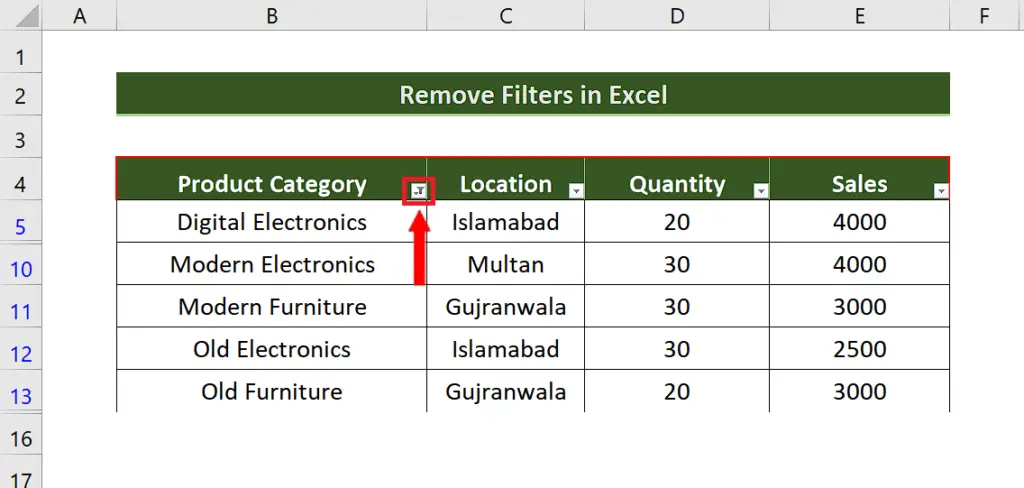
In today’s tutorial we’ll learn how to remove filters from the data. Let’s see the dataset above on which the filters have already been applied.
Now when we talk about removing the filters, it could mean two things,
- Clear the filter permanently from all of the data
- Clear only the current filter to apply a new one

In Excel, filters can be used to quickly sort and narrow down large amounts of data. They allow you to display only the rows that meet certain criteria, while hiding the rest of the data. Filters can be applied to columns in a table or data range and can be used in combination with other filters to create more complex queries.
Step 1 – Remove the filter from Data Tab
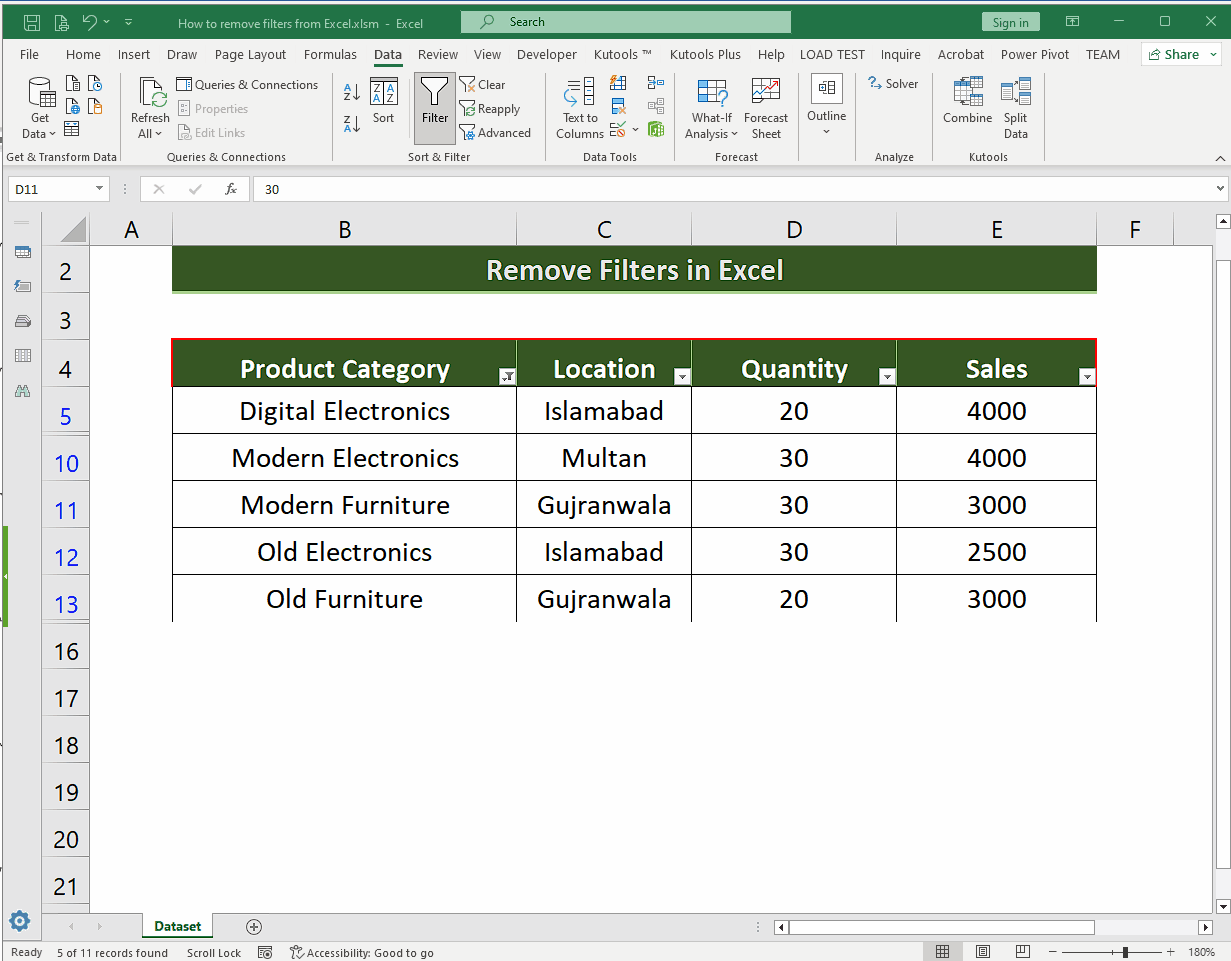
– Select a cell inside your dataset.
– On the list of main tabs, click on the Data tab.
– In the Sort & Filter tab, click on the Filter action button. This will remove the filter from all the data.
– Alternatively, you can also use the shortcut key to remove the filter from the dataset by pressing CTRL+SHIFT+L.
– This will remove the filter from all columns in the data range automatically.
Step 2 – Clear the current Filter only and apply a new one
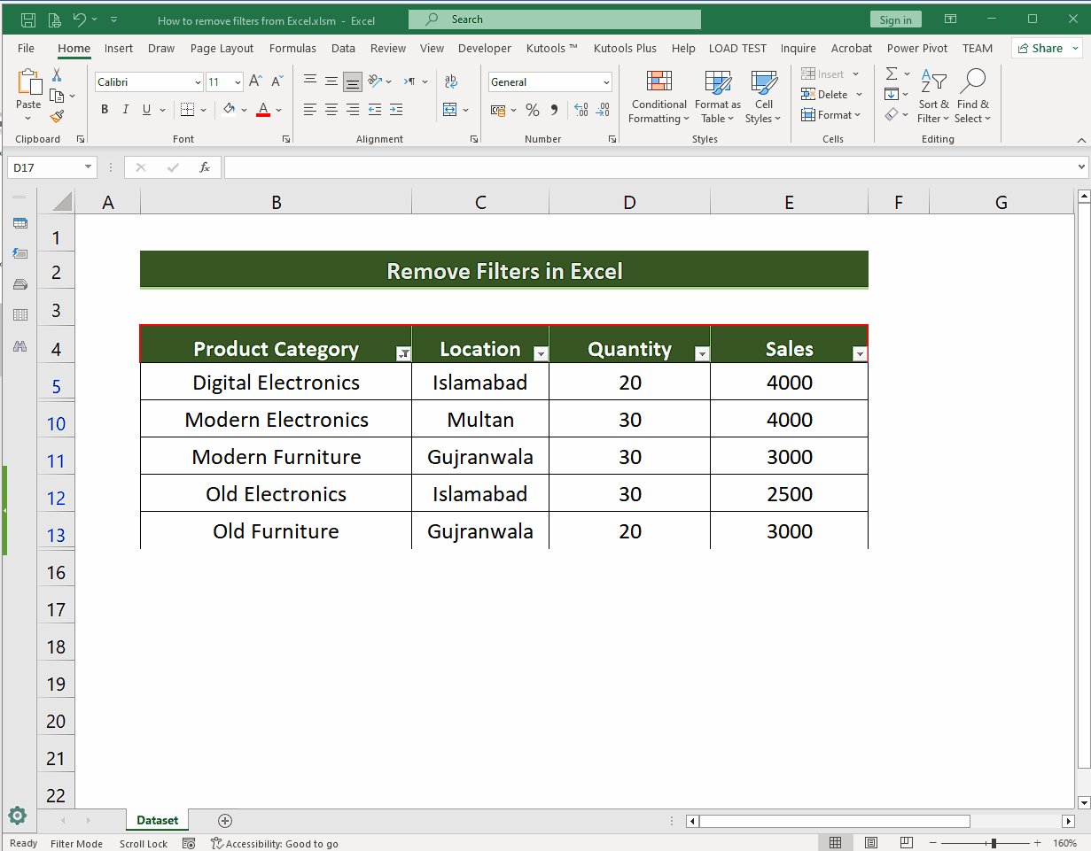
– We’ll go to the column header of interest, which in our case is the Product Category, because the filter is applied on this column, and click on the dropdown arrow.
– This will open up new options and we’ll click the Clear Filter from Product Category option this will remove the current filter and we’ll be able to see the complete data now.
– We can also do the same thing by clicking on the Data tab from the list of main tabs.
– Then in the Sort & Filter group, click on the Clear action button. This will remove the current filter from the data.
– We can apply a new filter as well as per our requirements as shown above.


