
How to Copy Conditional Format in Google Sheets
 By
SpreadCheaters
By
SpreadCheaters
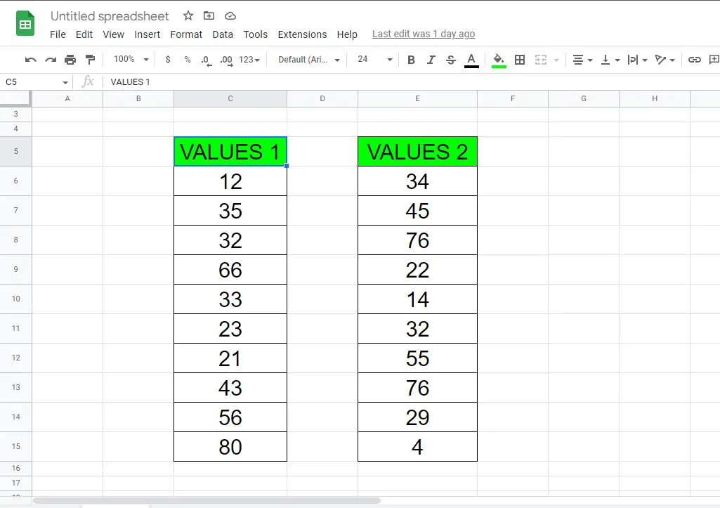
In this tutorial we have a Dataset above which contains 2 columns (Values 1, Values 2) with different values. We will apply the conditional format to the “Values 1” column and copy it to the “Values 2” column. Values less than 50 will be shown in darker color as compared to other values.
Conditional formatting is a powerful tool in Google Sheets that allows you to highlight specific data based on certain conditions. Whether you’re using it to flag errors, identify trends, or draw attention to important data, conditional formatting can be a real time-saver, but what if you need to apply the same formatting to multiple cells or ranges? Google Sheets makes it easy to copy conditional formatting.
Step 1 – Open Conditional Formatting.
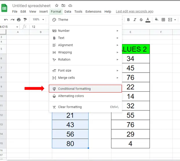
– First of all select the cells you want to apply conditional formatting on.
– Go to the Format tab and click on Conditional Formatting.
Step 2 – Apply the rule for Formatting.
– In the Format rules group open the drop down menu and choose the condition.
– In our case It will be Less than.
– Now enter the value according to the condition.
– In our case the value will be 50.
Step 3 – Copy Conditional Formatting for other cells

– After applying the format click the cell with format.
– Choose the Paint Format icon.
– Now select the cells where you want to paste the Conditional Formatting too.


