
How to condense data in Excel
 By
SpreadCheaters
By
SpreadCheaters
In Excel, condensing data can refer to the process of removing blanks or empty cells within a dataset. By removing blanks, users can ensure that their calculations, charts, and analysis are based on complete and contiguous data. This can be achieved by using filtering or sorting functions to exclude or delete rows or columns with blank cells, resulting in a more organized and efficient dataset for further analysis or presentation.
This post will outline the steps to shorten a list without leaving out any important information. Let’s follow the steps described below to learn the method to do it.
Step – 1 – Select a cell in the data
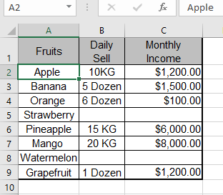
– Suppose we have the following data set to condense.
– The cursor must be on any cell of the dataset, ensure not on the blank cell.
Step – 2 – Go to the Data tab
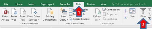
– Navigate to the Data tab in Excel.
– Click on the filter command button to apply a filter on our data set as shown in the image.
Step – 3 – Filter Applied to the dataset
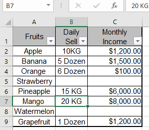
– The filter will be enabled for the dataset. Now we can choose any filter of our choice depending on the requirement.
Step – 4 – Choose Filter
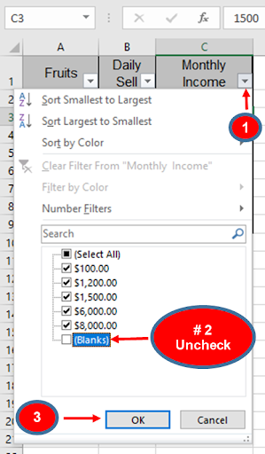
– Click on the drop-down arrow as marked in red.
– Uncheck the blanks from the data.
– Finally, click on the “OK” button.
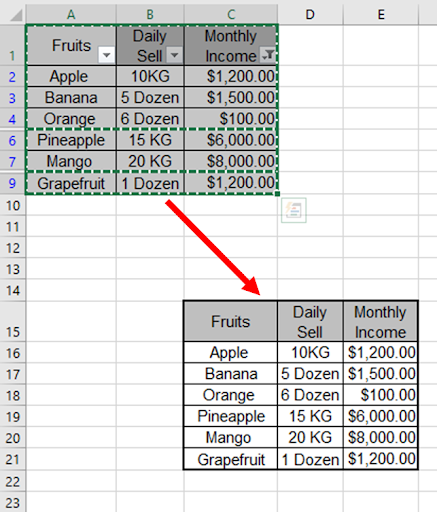
Step – 5 – Data Condensed
– We can observe that our dataset contains no blank cells.
– Copy all and paste them into another column.
– The data is condensed now with no blanks as shown in the image.


