Google Sheets is one of the best tools which is simple to use yet it provides so many features to handle, manipulate and perform simple to complex calculations on any type of dataset. It also provides many built-in tools and features that can help the data analysts in visualizing data in the best possible ways. One such feature is the ability of Google Sheets to apply filters on datasets to temporarily hide the unwanted information.

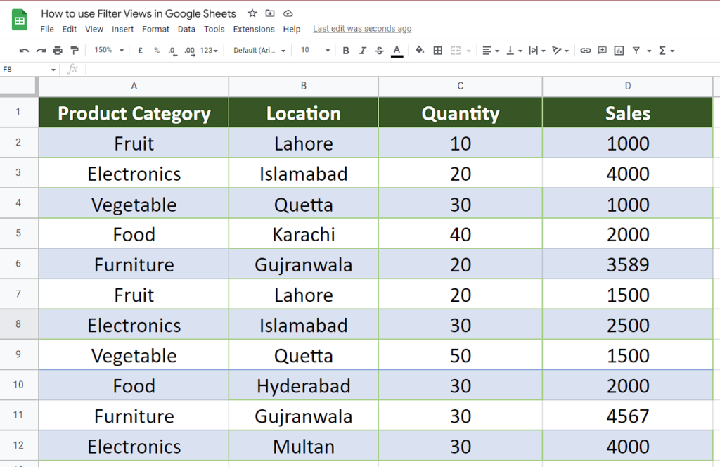
In today’s tutorial we are going to learn how to Filter Rows in Google Sheets. Let’s take a look at the following sales dataset.

Step 1 – Locate the Filter View Option in Data Tab to apply filter view

• Select a cell inside your dataset.
• Click on the Data tab on the main menu tabs. 
• Hover the mouse to Filter Views and there locate the Create new filter view.

This will apply a new filter view to the data. We can change the name and the range of the data as per our requirements.

There are three types of filters available in Google Sheets which are listed below;

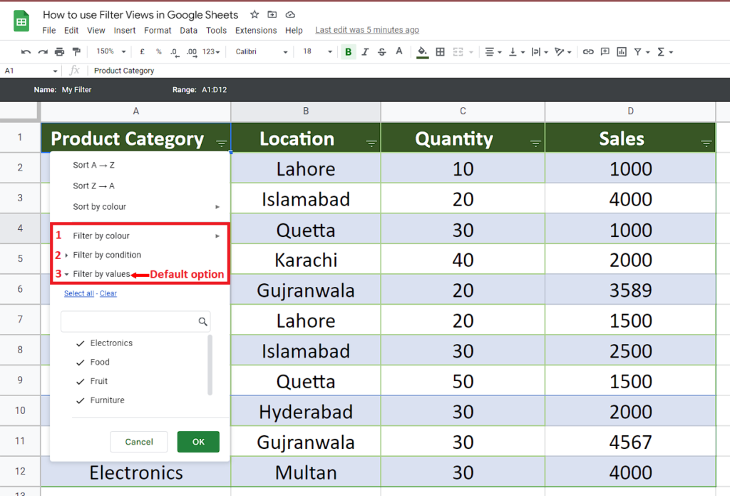
• Filter by Values (Default option)
• Filter by condition
• Filter by colour

Method 1 Filter by values:

Now that we have applied the filter view to our data, we can use it as per our requirements to see only the data that we are interested in. Let’s assume that we wish to see the sales data of Fruit items only from the Product Category column. So, let’s use the filter options to get it done. We’ll use Filter by values for this purpose.

Step 1 – Use Filter by values to filter rows in Google Sheets

• We’ll go to the column header of interest, which in our case is the Product Category and click on the dropdown menu.
• This will open up new options and we will see that all items are selected. Click Clear all option to exclude all items.
• Now select only the specific item you want to see, and in our case, it is Fruit. So we’ll select Fruit which will display all rows of data which include Fruit.

• We can revert this back to normal just by clicking Select all option again.

Method 2: Filter by Condition

We can apply the filter using a special condition as well. There are a lot of options in this area which can be used as per requirements. Mainly it provides us with three types of conditions;

• Text Based
• Date Based
• Numeric Data Based

Let’s see how to use these in the steps below.

Step 1 – Choose an appropriate filter from Filters options

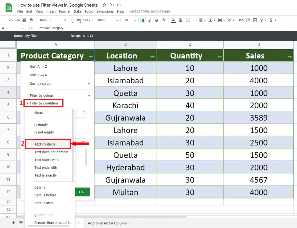
• To apply a text based filter, go to the Product Category column and again click on the drop-down menu.
• From the options available, click on the Filter by condition and then choose whatever filter that suits your requirement. In our case we’ll choose “Text contains” option.

Step 2 – Fill in Contains Filter options appropriately

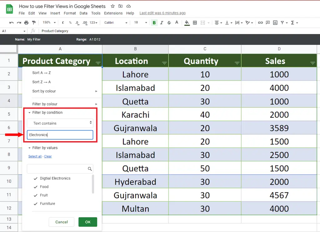
• The last step will open up a new option box to enter the criteria. You may fill in the box as per your requirements. However, we’ll search for all those items which contain the word Electronics in their description. So, fill in the options as shown in the picture above.

Step 3 – Apply the Filter conditions to filter rows

• After filling in the options properly, click the OK button.
• This will filter the data and we’ll get the rows, those items which contain the word Electronics in their description.

We can do the same thing with numeric data and dates as well. Let’s explore the filter by color option now.

Method 3: Filter by Colour

If our data has cells or rows filled with different colors then we can use this filter as well to get the respective data.

Step 1 – Apply the Colour Filter to get coloured rows only

• To apply a colour based filter, go to the Product Category column and again click on the drop-down menu.
• From the options available, hover the mouse on the Filter by colour option and then hover to Fill colour.
• Now choose the color as per your requirements and click on it. This will filter the rows by colour.