
How to color code Microsoft Excel cells based on values
 By
SpreadCheaters
By
SpreadCheaters
Color coding cells in Microsoft Excel involves automatically assigning distinct colors to cells based on their numeric or textual values. This formatting approach serves as a visual cue, enhancing the interpretation and analysis of data for improved efficiency.
In this tutorial, we will learn how to color code Microsoft Excel cells based on values. To color code cells in Excel the most common method is to utilize the built-in Conditional Formatting feature. By utilizing the conditional formatting feature we can easily color code cells based on custom rules according to the requirement.
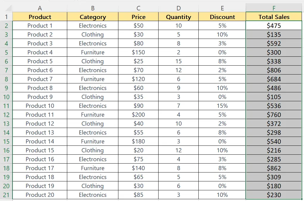
Let’s say we have sales data for some products. We want to color-code the sales that are above $300.
Method 1: Utilizing the Conditional Formatting
Step 1 – Select the Cells
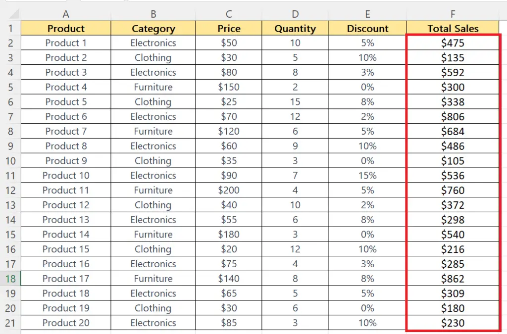
- Select the cells which you want to color code.
Step 2 – Perform a Click on the Conditional Formatting Button
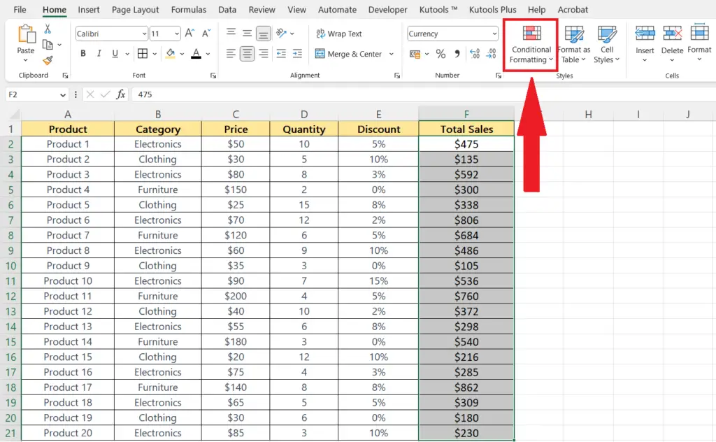
- Perform a click on the conditional formatting button in the Styles section of the Home tab.
Step 3 – Choose the “New Rule” Option
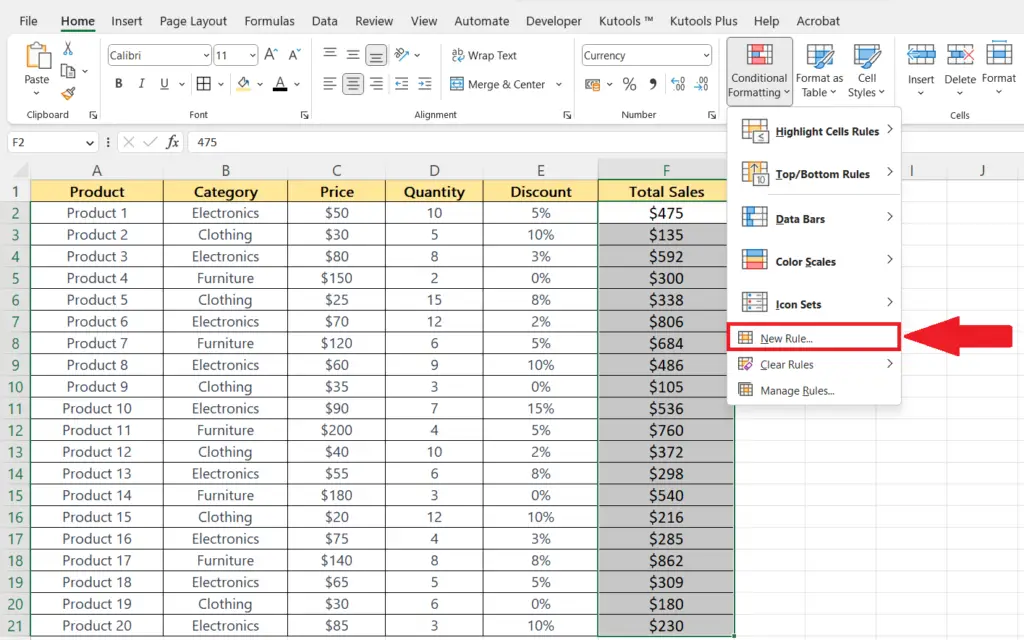
- Choose the “New Rule” option to create a customized rule based on your requirement.
- You may choose a built-in rule from the drop-down menu.
Step 4 – Choose the “Format only cells that contain” Option
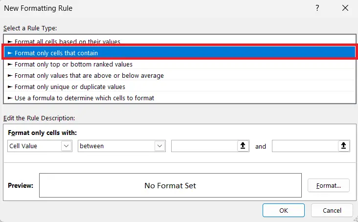
- Choose the “Format only cells that contain” option.
Step 5 – Set the Criteria in the “Format only cells with:” Section
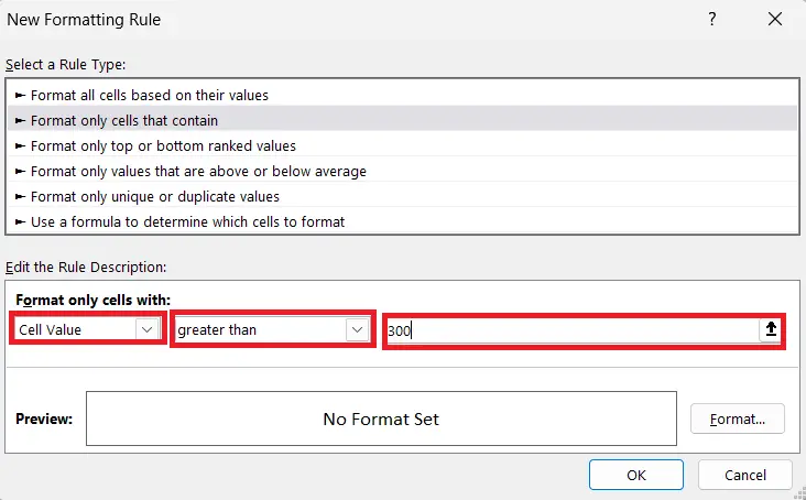
- Set the criteria.
- In this case, we will choose “Cell Value” in the first drop-down menu.
- Choose “greater than” in the second field.
- Now enter the value in the third field i.e. $300.
Step 6 – Perform a Click on the Format Button
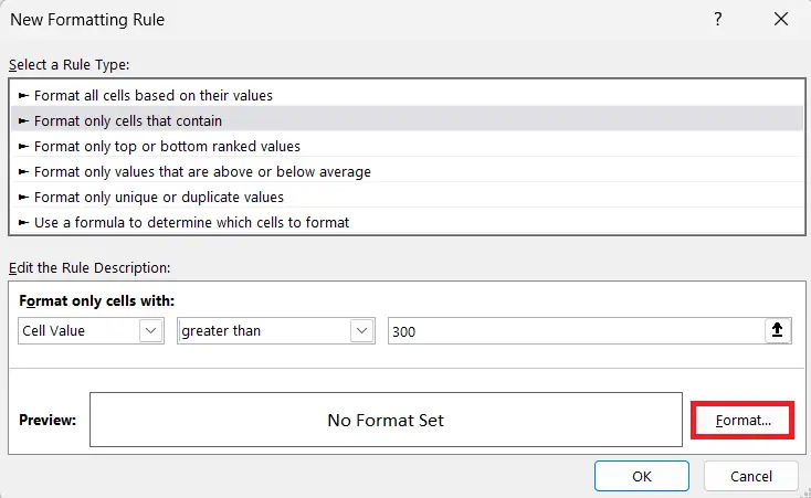
- Perform a click on the Format button.
Step 7 – Navigate to the Fill Tab and Choose the Color
- Navigate to the Fill tab in the dialog box.
- Choose the color.
- Perform a click on OK.
- The cells will be color-coded based on the set criteria.
Step 8 – Again Apply Conditional Formatting to Color Code the Cell with Values Less than $300
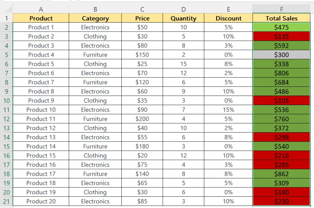
- Utilizing the same steps, format the cells that have a sales value of less than $300.
Method 2: Utilizing the Quick Analysis Tool
Step 1 – Select the Cells
- Select the cell which you want to color code.
Step 2 – Perform a Click on the Quick Analysis Tool Icon
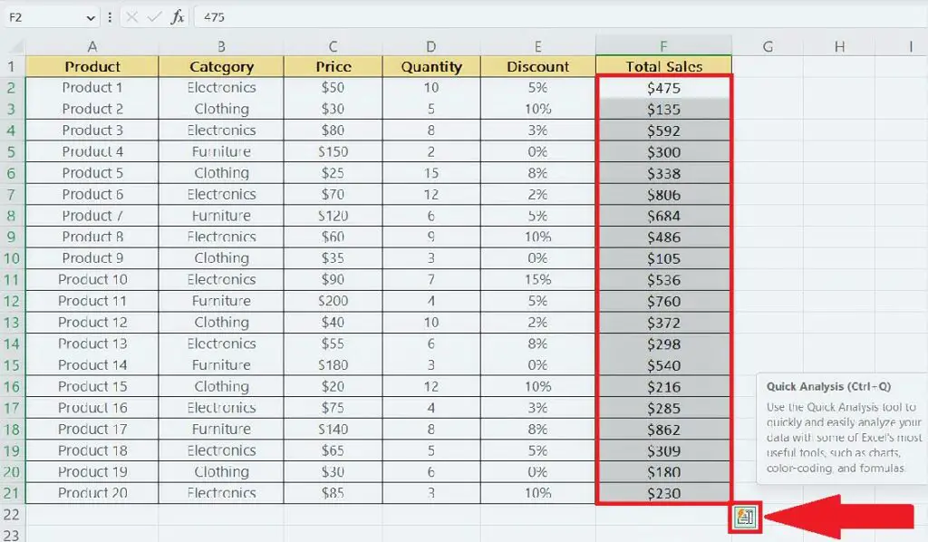
- Perform a click on the Quick Analysis tool icon that appears on the right end of the selection.
Step 3 – Choose the Color Scale Option
- Choose the Color Scale option from the menu.
- This formatting approach will apply a color gradient to the cells based on their values, ranging from red for the lowest values to green for the highest values.
Method 3: Utilizing the Find and Replace Feature
With the Find and Replace feature, it is possible to color code cells, but it is limited to text values only. To achieve this, we will use the same data set and apply color coding based on the category. The Electronics category will be colored blue, the Furniture category orange, and the Clothing category green.
Step 1 – Press the CTRL+H Keys
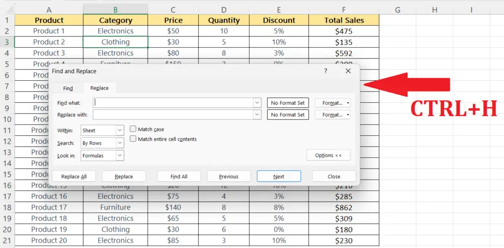
- Press the CTRL+H keys on the keyboard.
Step 2 – Input the Search Term in the “Find what” Field
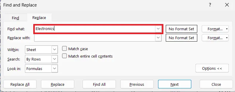
- Input the search term in the “Find what” field i.e. “Electronics”.
Step 3 – Input the “Replace with” Term
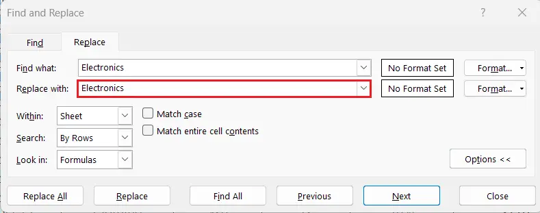
- Input the “Replace with” term i.e. “Electronics”.
Step 4 – Perform a Click on the Format Button for the “Replace with” Option
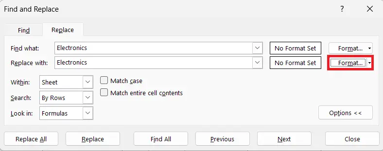
- Perform a click on the “Format” button for the “Replace with” option.
Step 5 – Navigate to the Fill Tab and Choose the Color
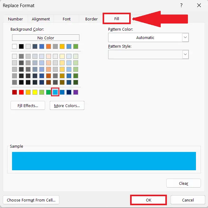
- Navigate to the Fill Tab.
- Choose the desired color i.e. we have selected blue for Electronics.
- Hit the OK button.
Step 6 -Click on the “Replace All” Button
- Perform a click on the “Replace All” button.
- All the cells with the specified term will be color coded.
Step 7 – Color Code Other Categories
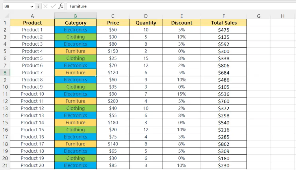
- Utilize the same steps to color code other categories i.e. Furniture and Clothing.


