
How to color code Google Sheets
 By
SpreadCheaters
By
SpreadCheaters
Color coding in Google Sheets means applying colors to the cells in a spreadsheet based on specific conditions or criteria. This can help you visually organize and highlight data, making it easier to understand and interpret at a glance.
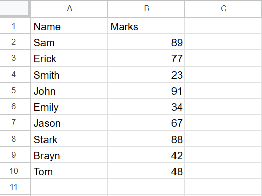
We have a dataset that includes student names along with their respective marks. Our task is to apply color codes to the marks based on their numeric values. Two methods are available for this task: the first involves using the color scale option, and the second involves using conditional formatting rules.
Method 1: Color code the cells using the Color scale option
Step 1 – Select the range of cells
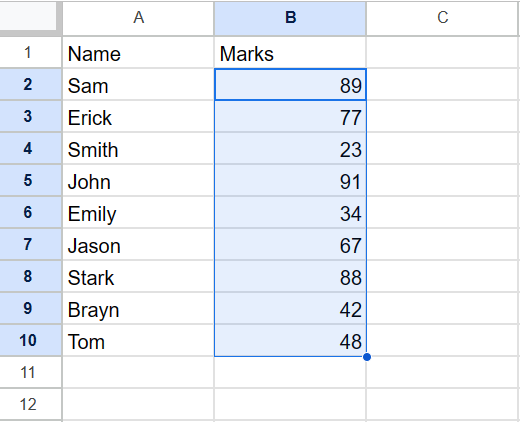
- Select the range of cells you want to color
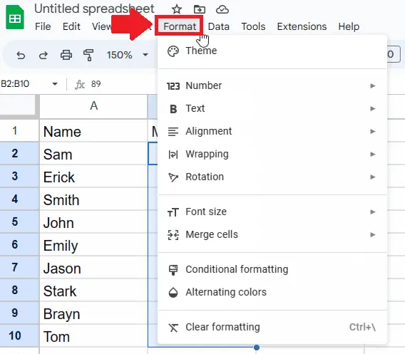
Step 2 – Click on the Format Tab
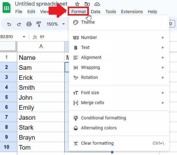
- After selecting the range of cells, click on the Format tab from the Taskbar, and a drop-down menu will appear
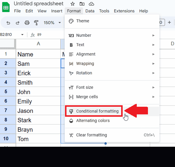
Step 3 – Click on the Conditional Formatting option

- From the dropdown menu, click on the Conditional Formatting option and a conditional formatting dialog box will appear on the right side of the page
Step 4 – Click on the Color Scale option
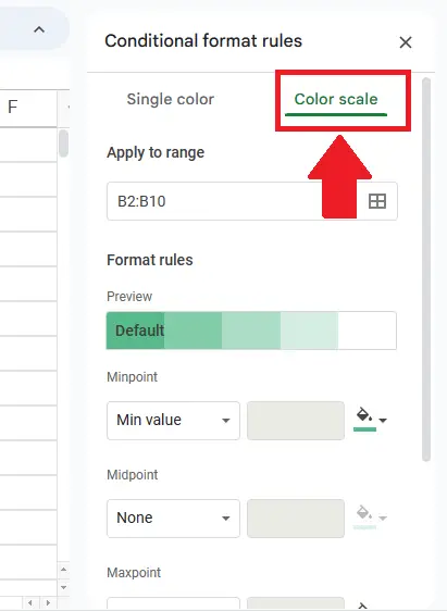
- From the Conditional Formatting dialog box, click on the Color Scale option at the top of the dialog box
Step 5 – Select the Colors
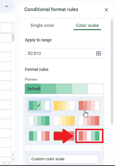
- Click on the box below the Preview option and a list of color ranges will appear
- From the list Click on the Color range you want
Step 6 – Select the Type of Values
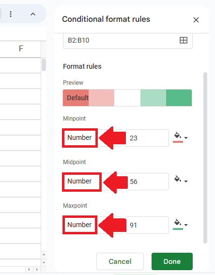
- Select the type of values in the box below Minpoint, Midpoint, and Maxpoint options
- Here we have selected numbers as the selected range of cells contains numbers
- You may select any other type according to your dataset
Step 7 – Click on Done
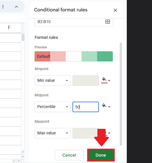
- Click on the Done option at the end of the dialog box to get the required result
Method 2: Color Code the cells by using the “is between” formatting rule
Step 1 – Select the range of cells

- Select the range of cells you want to color
Step 2 – Click on the Format Tab
- After selecting the range of cells, click on the Format tab from the Taskbar, and a drop-down menu will appear
Step 3 – Click on the Conditional Formatting option
- From the dropdown menu, click on the Conditional Formatting option and a conditional formatting dialog box will appear on the right side of the page
Step 4 – Select the Format Rule
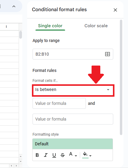
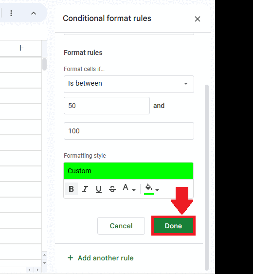
- In the box below the Format Cells option select the “Is Between” option
Step 5 – Select the Range of values
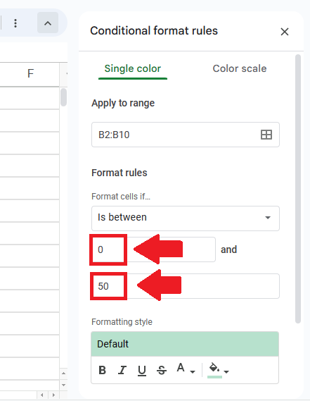
- To select the range of values type the lower value in the first box below Format cells if box
- Type the higher value of the range in the second box below Format cells if box
Step 6 – Select Color
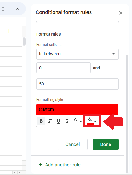
- After selecting the range, select the color from the box below the Formmating style option
Step 7 – Click on the Done option
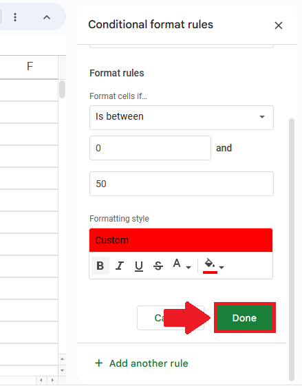
- After selecting the color, click on the Done option to apply the formatting
Step 8 – Click on the Add Another Rule option
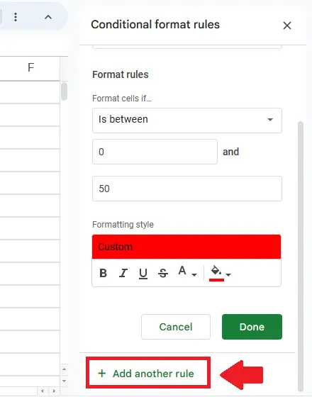
- After clicking on the done option, Click on the Add Another Rule option, and a new conditional formatting dialog box will appear
Step 9 – Select the Range of values
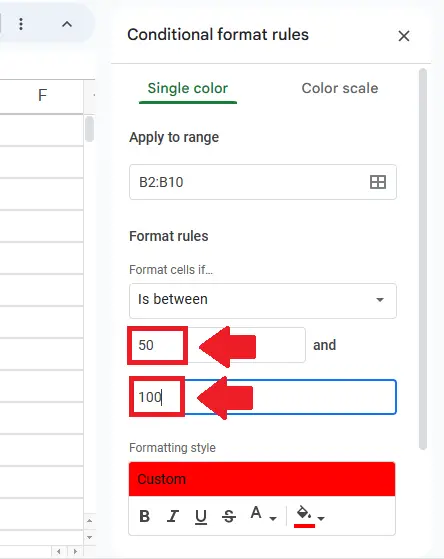
- To select the range of values type the lower value in the first box below Format cells if box
- Type the higher value of the range in the second box below Format cells if box
Step 10 – Select the Color
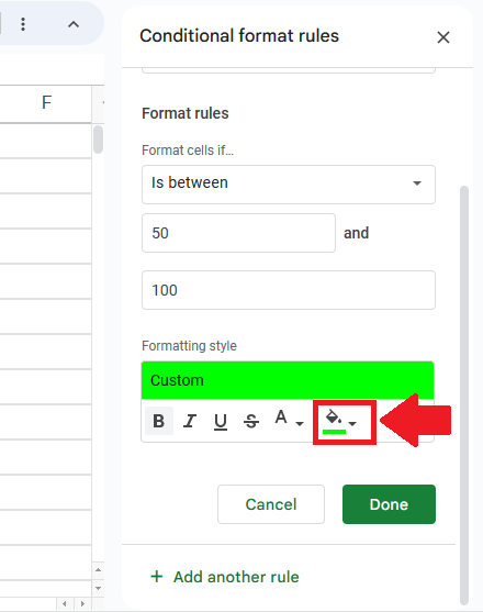
- After selecting the range, select the color from the box below the Formmating style option
Step 11 – Click on the Done option
- After selecting the color, click on the Done option to get the required result
Conclusion:
We have explained only two methods to use conditional formatting to color code the data. However, there are a lot of other ways which can be used to assign colors to data cells based upon a specific criteria. Therefore, you can use other cases or conditions from conditional foratting options and use multiple colors to differentiate data cells from each other.


