How to change the display of subtotals in the pivot table

Subtotals in a pivot table enable drill-down analysis, allowing you to examine the underlying details for each subtotal. By expanding or collapsing the subtotals, you can reveal or hide the individual records that contribute to the subtotal. This helps you investigate specific subsets of data and gain more insights into the factors driving the subtotal values. 

In this tutorial, we will learn how to change and display subtotals in the pivot table. Furthermore, adding subtotals in a pivot table helps organize and summarize your data, facilitates analysis, and improves the presentation of results, leading to better decision-making and understanding of the underlying data patterns.

There are two cases by which we can change the display of subtotal which are mentioned below;

Case 1 – Add subtotal in pivot table

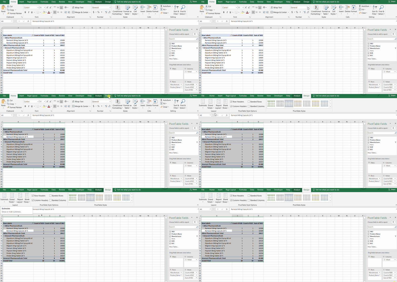
Whenever some data is placed over the worksheet and Pivot Table is created, the data doesn’t show the subtotals as default. The example is illustrated as under.

To solve this problem, the necessary steps are given as under.

Step 1 – Select the pivot table

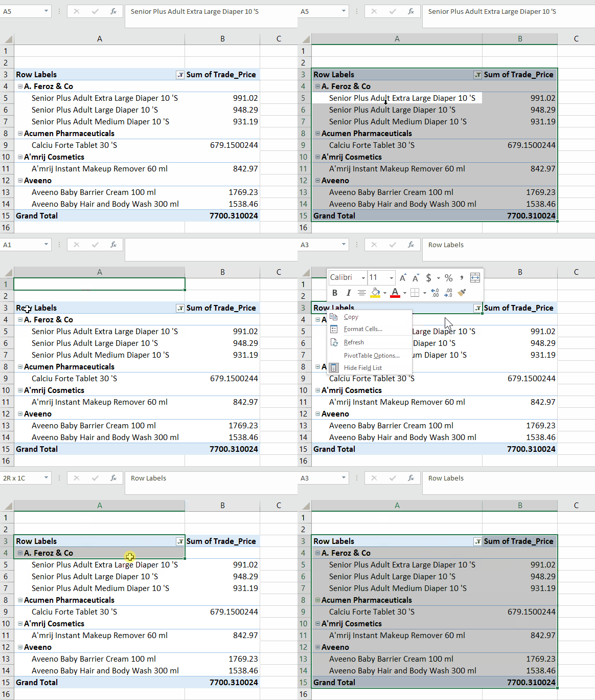
• Select any cell of the pivot table.
• Press the keyboard shortcut key Ctrl + A,  to select the whole pivot table data simultaneously. (OR) Click on the single cell and drag the mouse to select the complete pivot table. As shown above;

Step 2 – Go to the Design tab

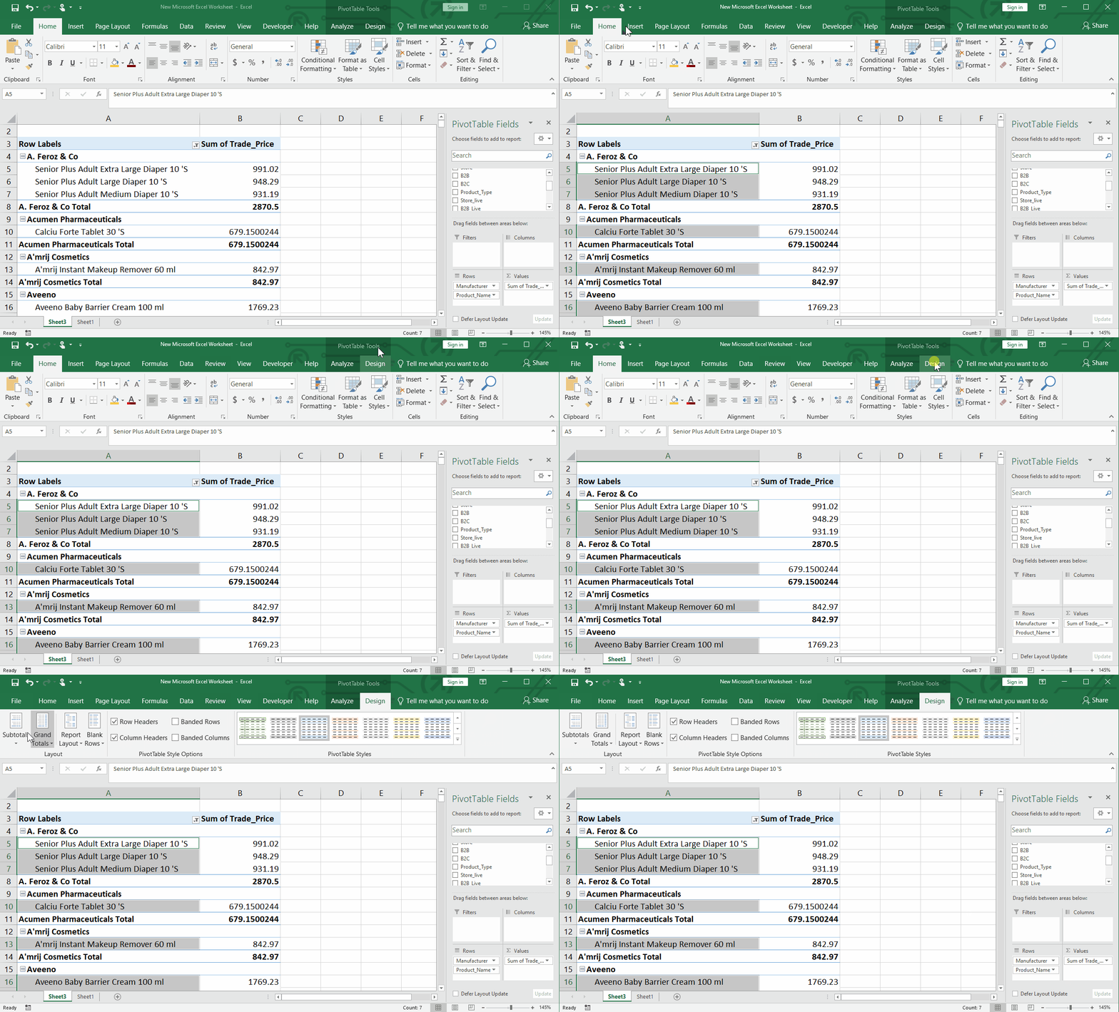
• In the PivotTable Tool, Click the Design tab.
• In the Layout section, Click on Subtotals. As shown above;

Step 3 – Select the subtotal

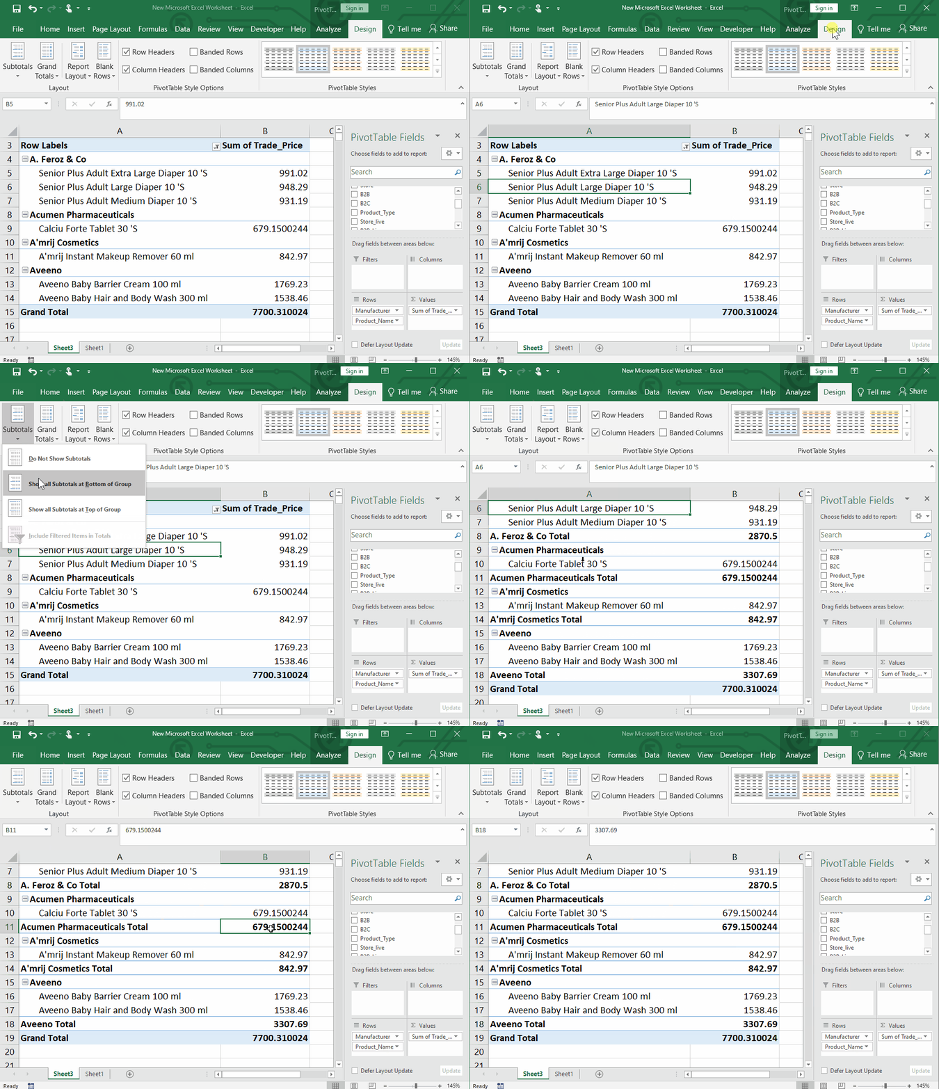
• As we click on the subtotal, a dropdown menu will appear.
• Click on Show all subtotals at the Bottom of the Group
•  The subtotals will be calculated and displayed at the bottom of each head. As shown above;

Case 2 – Disable subtotal in pivot table

In this case, we are assuming that the data already show the subtotals and we want to hide the  subtotals now. So, we will disable the subtotal by following the steps explained below;

Step 1 – Select the pivot table

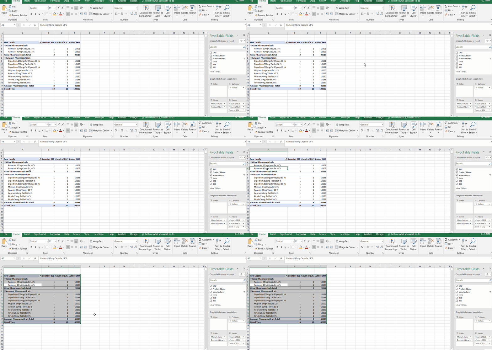
• Select any cell of the pivot table.
• Press the keyboard shortcut key Ctrl + A,  to select the whole pivot table data simultaneously. (OR) Click on the single cell and drag the mouse to select the complete pivot table. As shown above;

Step 2 – Go to the Design tab

• In the PivotTable Tool, Click the Design tab.
• In the Layout section, Click on Subtotals. At the left corner. As shown above;

Step 3 – Select the subtotal option

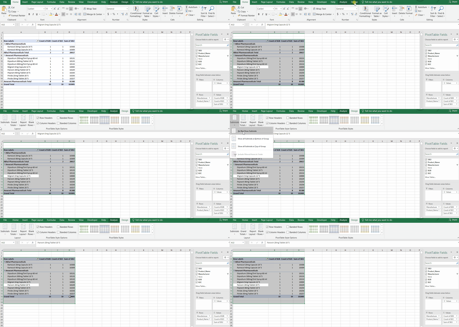
• As we click on the subtotal, a dropdown menu will appear.
• Click on Do not show subtotals.
•  The subtotals will be disabled and only the grand total will be visible. As shown above;

Conclusion:

Hence, by using the above-shown method we are now able to add and disable subtotal of each category. When you create a PivotTable that shows value amounts, subtotals, and grand totals appear automatically.