How to change the column name in Excel 

Excel’s column names are alphabetized by default. The contents of a column are not indicated by the column’s name. As a result, you frequently rename the column to suit your convenience. Excel uses numbers to designate rows while using alphabets to denote columns. Additionally, rows can have their names changed. 

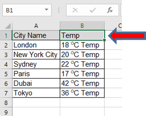
It is possible to rename a column in Excel for any reason. The steps for renaming a column in Excel are covered in this section. If we select Column B1, Let’s examine how we can change the name of this column. 

Method 1  – Rename the column with a display bar. 

Step – 1 – Select the Column 

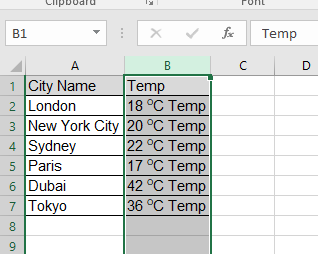
• Select the column which we need to rename. 
• Suppose below screen. 

Step – 2 – Delete the column name from the bar 

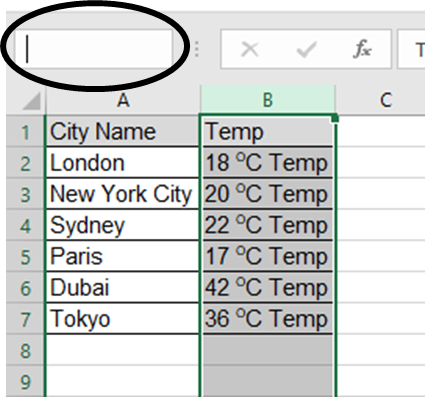
• Delete the Column Name from the bar under circle as shown in the screen. 

Step – 3 – Enter the desired column name in bar 

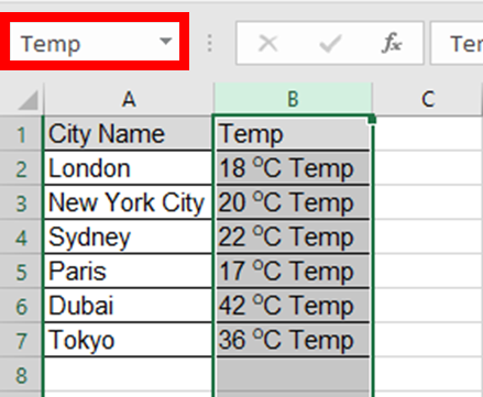
• Enter the column name. We’ll add “Temp” in this example. 

• Press the ENTER key now. 
• We can observe that Temp has been added to the recommended Column. 

Method 2 – Rename the column with Advance Option. 

This solution merely demonstrates how to conceal the standard column and row names. In addition, you can modify the dataset heading. In this case, Excel’s Advanced option will be used. To do this, take these actions: 

Step – 1 – Click to the first Row of the data set 

• To add a new row atop the current row, click the first row of the sheet. 

Step – 2 – Go to the File tab 

• Click on File tab first. 
• Select Options from the menu. 

Step  – 3 – Click on the Advanced option 

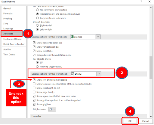
• Click on the advance option, then scroll down on “Display option for this worksheet”. 
• Uncheck the desired option as shown in screen. 

• Press “OK” button 

Step – 4 – Applied condition outcome  

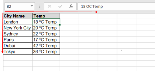
• We can see, the column name is the dataset header now and the column letters and row numbers are not visible any more.