How to change cell colour based on value In Google Sheets

Google Sheets conditional formatting is a feature to automatically change the font properties of a specific cell, row, column, and even the background colour of the cell, based on rules you set. In other words, this tool uses the power of visualisation to make your data stand out. By colouring cells, you highlight specific values, making them easier to view, and easier to understand complex tables.

Conditional formatting can be used in practically any workflow to visualise information: patterns of data, trouble spots, good news, or even faulty or flawed data. It is possible that no other Google Sheets tool can be used in so many applications.

Before getting into detail, it is important to understand that any work with conditional formatting follows the same pattern, which has three key elements:

• Range: This is a cell or cells to which the rule should be applied. 
• Rules or Trigger: It defines the condition for the rule to be used. For example, the trigger can be Less than.
• Style: When the rule is applied, it changes the cell to a style of your choosing.

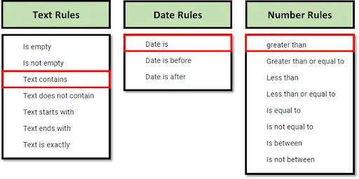
To understand the conditional formatting rules better, we will divide the rules in 03 groups.

• Text Rules.
• Date Rules.
• Number Rules.

Let’s discuss the highlighted rules one by one.

Method 1 – Conditional Formatting Thru Text Rules

Although Text rules suggest they can only be applied to text-formatted cells, we can actually use them on any kind of cell.

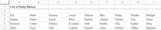
For example, let’s identify the baby names containing “an” in the following data above.

Step 1 – Select Data Range

• With the help of the selection handle, select data in the table.

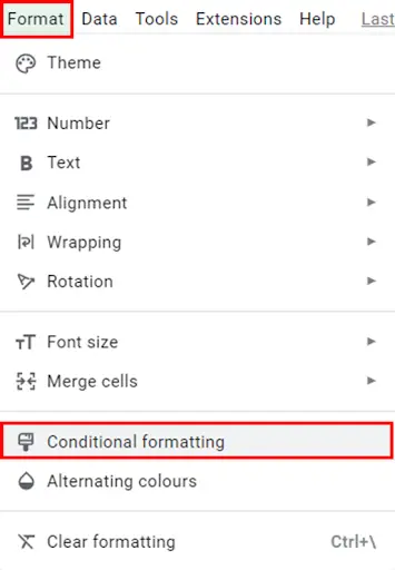
Step 2 – Click on Format Menu

• Click on the format menu.

Step 3 – Select Conditional Formatting

• Select conditional formatting.
• Conditional formatting screen will appear at the right side of your screen.

Step 4 – Select Conditional Formatting Rule

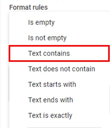
• We have already selected the range. Now, simply select the formatting rule under Format rules sections.

.

Step 5 – Cell Formatting Condition

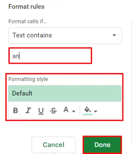
• As we want to highlight baby names having “AN” in the spelling. Type “AN”.
• Select your desired Formatting style. For this example we are moving on with the default style.
• Click on the Done button.

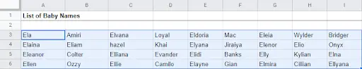
Step 6 – Highlight Cells Using Text Rule

• When you press the Done button, the cells satisfying the above selected condition will be highlighted automatically as shown above.

Method 2 – Conditional Formatting Thru Date Rules

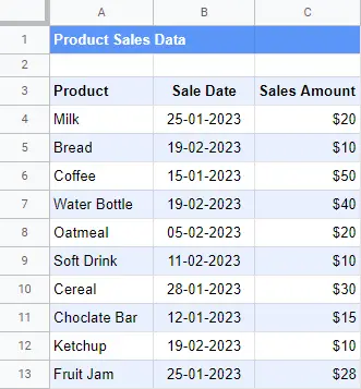
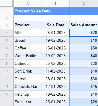
Let’s assume that we have sales data of a store. To highlight today’s date, follow these steps.

Step 1 – Select Data Range

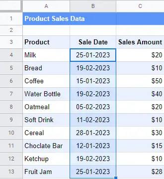
• With the help of the selection handle, select data in the table.

Step 2 – Click on Format Menu

• Click on the format menu.

Step 3 – Select Conditional Formatting

• Select conditional formatting.
• Conditional formatting screen will appear at the right side of your screen.

Step 4 – Select Conditional Formatting Rule

• Date range is already selected. Select the formatting rule under Format rules sections.

Step 5 – Cell Formatting Condition

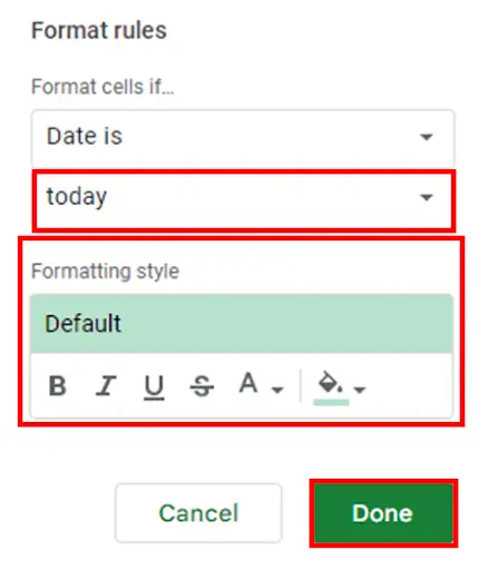
• We want to highlight today’s date. Select today from the drop down menu.
• Select your desired Formatting style. For this example we are moving on with the default style.
• Click on the Done button.

Step 6 – Highlight Cells Using Date Rule

• When you press the Done button, the cells satisfying the above selected condition will be highlighted automatically as shown above.

Method 3 – Conditional Formatting Thru Number Rules

Let’s assume that we have sales data of a store. To highlight sales value with greater than condition, follow these steps.

Step 1 – Select Data Range

• With the help of the selection handle, select data in the table.

Step 2 – Click on Format Menu

• Click on the format menu.

Step 3 – Select Conditional Formatting

• Select conditional formatting.
• Conditional formatting screen will appear at the right side of your screen.

Step 4 – Select Conditional Formatting Rule

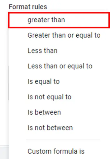
• Range is already selected. Select the formatting rule under Format rules sections.

Step 5 – Cell Formatting Condition

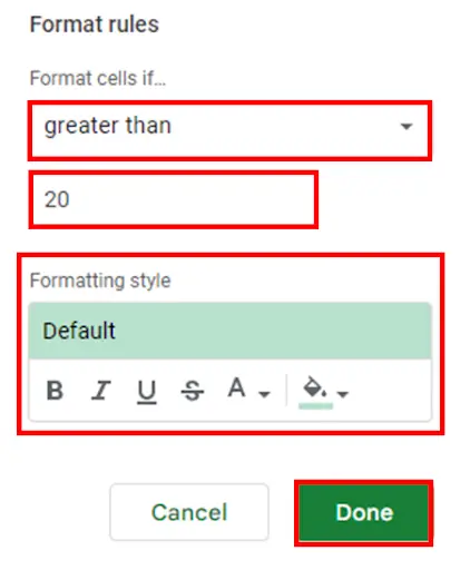
• To find out the sales value greater than 20. Type 20 as the condition to highlight the cell(s).
• Select your desired Formatting style. For this example we are moving on with the default style.
• Click on the Done button.

Step 6 – Highlight Cells Using Number Rule

• When you press the Done button, the cells satisfying the above selected condition will be highlighted automatically as shown above.