How to calculate percentile in Google Sheets

In this modern age of the world, people often require different smart techniques for the interpretation and analysis of data. In Google Sheets, the percentile is one of the convenient tools that is used to summarize and contrast distinct values in a dataset. By calculating percentiles, one can easily evaluate performance, track progress, interpret data, and make comparisons. It is very effective to use while handling a large set of data. It is very important to know that percentiles are different from percentages. Percentile indicates a relative position within a dataset, while percentage represents a proportion or ratio out of 100.

In today’s tutorial, we’ll learn how to calculate percentile in Google Sheets. Let’s examine the following cases for the calculation of percentiles.

CASE 1 – Calculation of n-th percentile in a data set

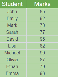
Following is a data set containing the marks of students in a class test:

From the above data, we can calculate any nth percentile of the data set. For example, a teacher wanted to calculate the 65th percentile of the marks of students in the class test. So, for the evaluation of the 65th percentile, we’ll consider the following steps: 

STEP 1 – Label a column for the calculation of percentile

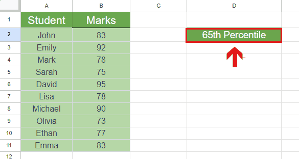
• Move your cursor to the cell which you want to label.
• Label the cell with the heading “65th Percentile”.

STEP 2 – Apply the formula 

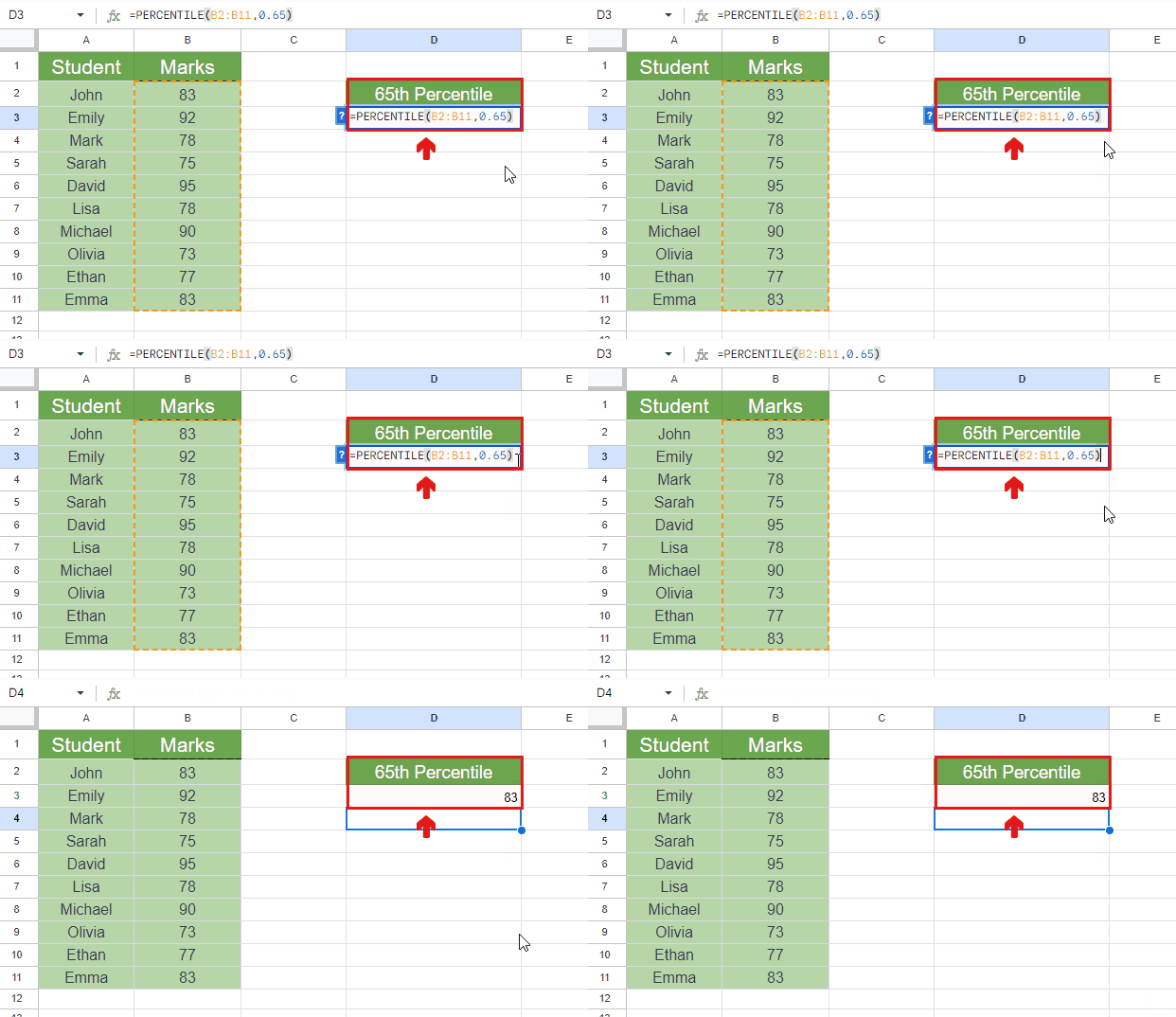
• For the calculation of the 65th percentile of the given data, the required formula is:

                                             =PERCENTILE(B2:B11,0.65)

• Write the above formula in the cell, below the heading.
• Press Enter key to put the formula into working.
• The 65th Percentile of the given data will be calculated.

RESULT: The 65th percentile of the data is 83, which is the mark of John. It means that John scored higher than 65% of the class students.

CASE 2 – Calculation of percentile for single values

We can calculate the percentile of individual values to analyze and compare it with other values of the data set. For the calculation of percentile, we’ll consider the same data set as in the above case.

Following are the steps for the evaluation of percentile:

STEP 1 – Create a column for the calculation of percentiles

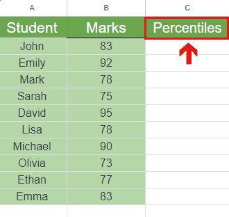
• Move your cursor to the first cell of the next column
• Label it with the heading “Percentiles” 

STEP 2 – Apply the formula for the calculation

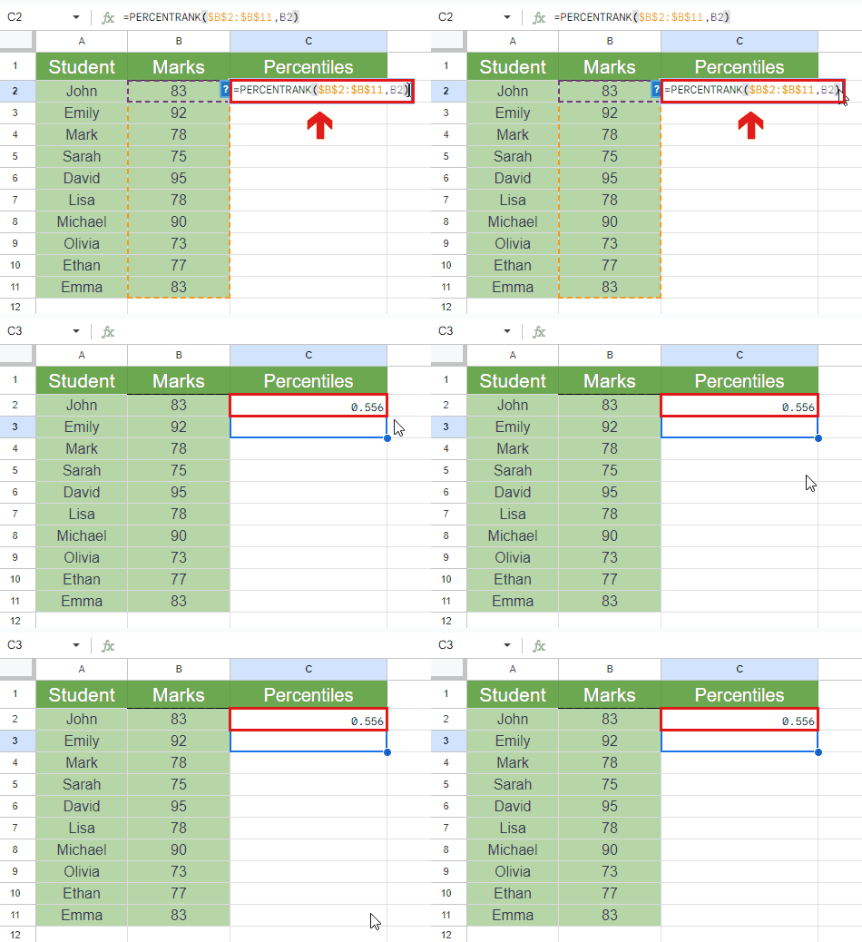
• Move your cursor to the cell below the heading.
• The required formula for the calculation of the percentile of one value, say B2 with respect to other values is:

                             =PERCENTILERANK($B$2:$B$11,B2)

• Note down the above formula in the cell.
• Press Enter key.
• The percentile will be calculated.

STEP 3 – Use the AutoFill Handle to calculate the percentiles of all values

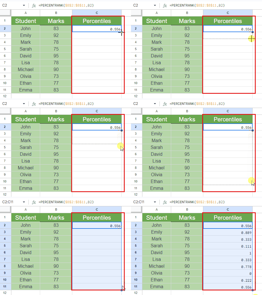
• Move your cursor to the cell in which the percentile of the first value is calculated.
• Select the cell and move the cursor to the lower right corner of the cell.
• Drag the AutoFill Handle to the last cell containing the value.
• The percentiles of all the values will be calculated.

STEP 4 – Conversion of decimal into percentage

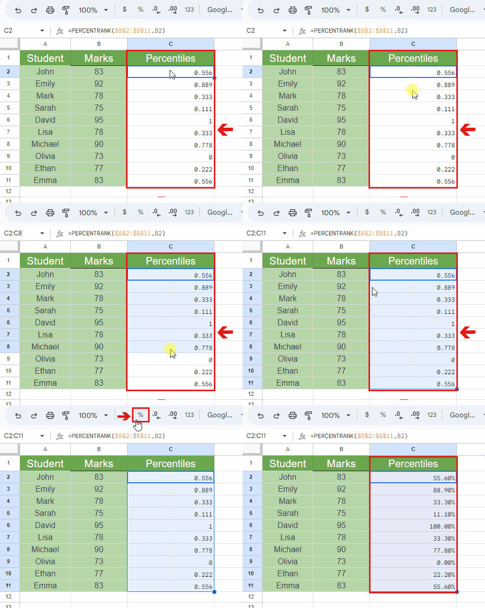
If you want to convert the decimal form of percentiles into percentages, then you should follow these steps:

• Select the column that contains all the percentiles.
• Click on the “%” icon on the above panel.
• All the percentiles in decimal will be converted into percentages.

Note: 

The 0th percentile in the dataset represents the lowest value and the 100th percentile represents the highest value in the dataset.