How to calculate percentage change in Google Sheets

Percentage change in Google Sheets is a powerful tool that provides valuable insights into data trends. Whether you are analyzing sales figures, website traffic, or any other metrics, calculating percentage change can help you to understand how things are evolving over time. Percentage change makes it easier to compare data over different time periods or between different data sets, as it provides a consistent basis for comparison. 

In this tutorial, we will learn how to calculate percentage change in Google Sheets. In Google Sheets, we can calculate percentage change by subtracting the old value from the new value and dividing the result by the old value. The formula is (new value – old value) / old value. Then we can format the cell as a percentage to convert the decimal value to a percentage. To avoid negative signs for decreases, we can use the ABS function.

Currently, we have a data set in which the sales of some products for the two years i.e. 2020 and 2021 are listed. We will calculate the percentage increase or percentage decrease for the sales of each product.

Method 1: Calculating percentage change using Generic Formulae

Step 1 – Select a Blank Cell and Place an Equals Sign

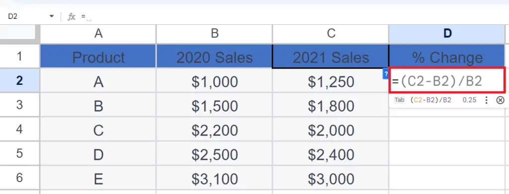
• Select a blank cell where you want to calculate the percentage change.
• Place an Equals sign in the first cell. You will notice that Google Sheet’s AI automatically detects your intention and suggests you the formula that can be used to calculate the percent change as shown above.

Step 2 – Enter the Formulae for Percentage Change

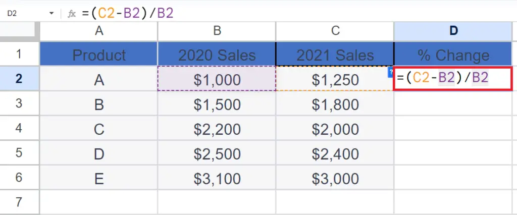
• We can see that the formula suggested by Google Sheets was correct so, we’ll use the same formula for percentage change, which is as follow; 

            (C2 – B2) / B2

Where C2 is the cell representing the new sales i.e. for the year 2021.

B2 is the reference of the cell containing the old sales i.e. for the year 2020.

Step 3 – Press the Enter Key

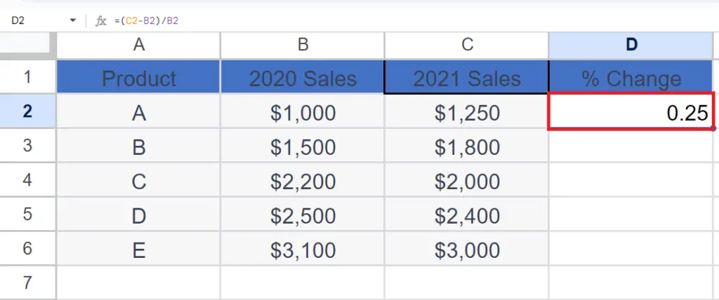
• Press the Enter key.

Step 4 – Change the Format

• Change the format of the cell to percentage format using the Percentage Style button in the Number section in the Home tab or we can use the CTRL+SHIFT+% shortcut keys.

Step 5 – Use Autofill to Calculate Percentage Change for Each Product

• Use Autofill to calculate the percentage change for each of the listed products.

Method 2: Calculating percentage change using ABS Function

Step 1 – Select a Blank Cell and Place an Equals Sign

• Select a blank cell where you want to calculate the percentage change.
• Place an Equals sign.

Step 2 – Enter the Formulae with ABS Function for the Percentage Change

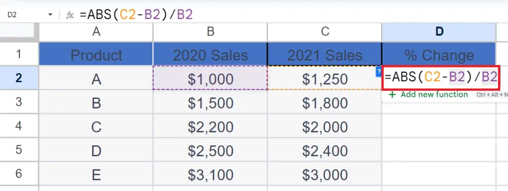
• The syntax will become:

            ABS(C2 – B2) / B2

Where C2 is the cell representing the new sales i.e. for the year 2021.

B2 is the reference of the cell containing the old sales i.e. for the year 2020.

Step 3 – Press the Enter Key

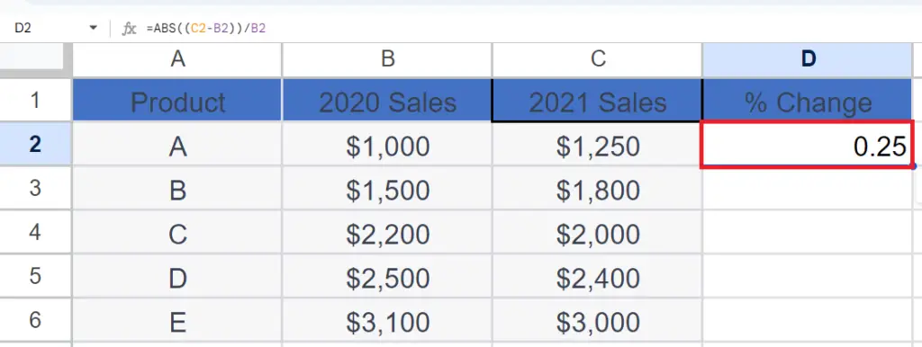
• Press the Enter key.

Step 4 – Change the Format

• Change the format of the cell to percentage format using the Percentage Style button in the Number section in the Home tab or we can use the CTRL+SHIFT+% shortcut keys.

Step 5 – Use Autofill to Calculate Percentage Change for Each Product

• Use Autofill to calculate the percentage change for each of the listed products.

Conclusion:

Based on the presented methods, it can be concluded that the first approach is more pragmatic as it calculates the percentage change and presents the result with discernible positive and negative signs. This feature enables a lucid understanding of the percentage increase or decrease in the values. In particular, the presence of a positive sign implies an increase in the value, whereas a negative sign indicates a decrease.