How to calculate IRR in Microsoft Excel for monthly cash flow

The Internal Rate of Return (IRR) is a robust financial measure employed to evaluate the profitability and desirability of an investment. It signifies the rate at which an investment’s net present value (NPV) reaches zero.

This article will teach us how to calculate IRR in Microsoft Excel for monthly cash flow. Excel provides a convenient IRR function to calculate the IRR quickly and accurately. In this article, we will explore how to calculate IRR in Excel specifically for monthly cash flows.

Method 1: Utilizing the IRR Function

The most common and simplest method to calculate “The Internal Rate of Return” is with the help of the IRR function.

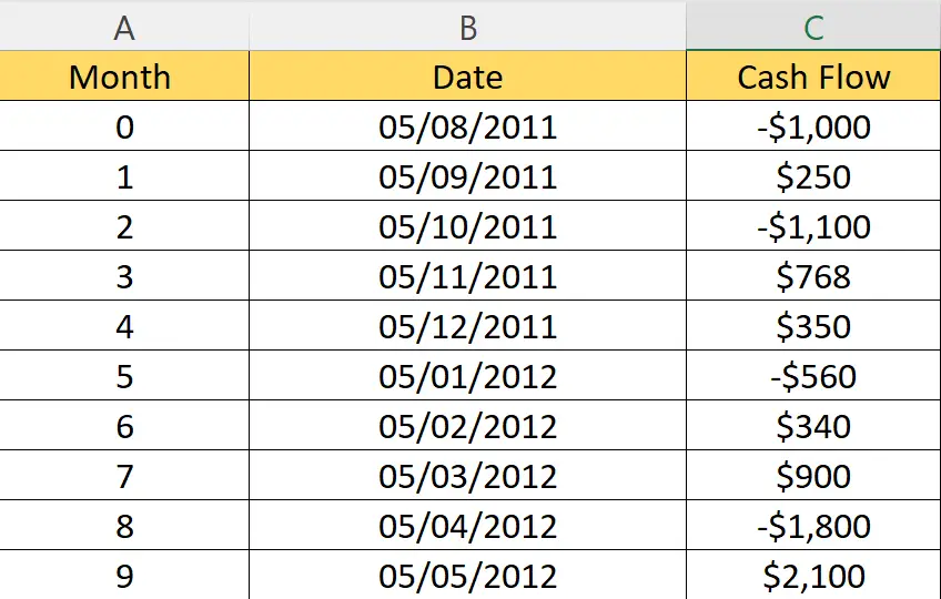
Step 1 – Organize the Data

• Organize the data i.e. cash flow for each month in a column.

Step 2 – Utilize the IRR Function

• Utilize the IRR function.

• Where C2:C11 is the range containing the cash flow for each month.
• Hit the Enter key.

Method 2: Calculating IRR with the XIRR Function

To determine the Internal Rate of Return (IRR) for monthly cash flows in Excel, you can employ the XIRR function, which accounts for irregularly timed cash flows. This function is specifically designed to handle monthly or other uneven intervals between cash flows. Here is a step-by-step guide on how to calculate IRR using XIRR in Excel:

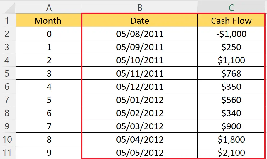
Step 1 – Organize the Data

• Organize the data into columns.
• For the XIRR function, we have to provide the dates for each period thus, the dates should also be organized in a column in addition to the cash flow.

Step 2 – Utilize the XIRR Function

1. Utilize the XIRR function in a blank cell.

• The first parameter is the range containing the cash flow.
• The second parameter is the range containing dates.
• Hit the Enter key.
• The function will return the Internal Rate of Return, but it would be more accurate than the IRR function.