How to calculate the risk-free rate in Microsoft Excel 

Calculating the risk-free rate is an important step in finance and investment analysis. The risk-free rate is the theoretical rate of return on an investment that carries zero risk. It is often used as a benchmark for other investments and is a key component in various financial models.

In this tutorial, we will learn how to calculate the risk-free rate in Microsoft Excel. There are several methods for calculating the risk-free rate including Treasury Yield, Historical Returns, and Market Risk Premium. The Treasury Yield method involves finding the yield on a Treasury security, while Historical Returns use past returns on safe investments. Market Risk Premium calculates the additional return an investor expects to receive over the risk-free rate to compensate for taking on the risk of investing in the stock market.

Method 1: Treasury Yield

Suppose you want to calculate the risk-free rate for a 10-year investment. You go to the Treasury Department’s website and find that the yield on a 10-year Treasury bond is 1.7%. 

Step 1 – Select a Blank Cell

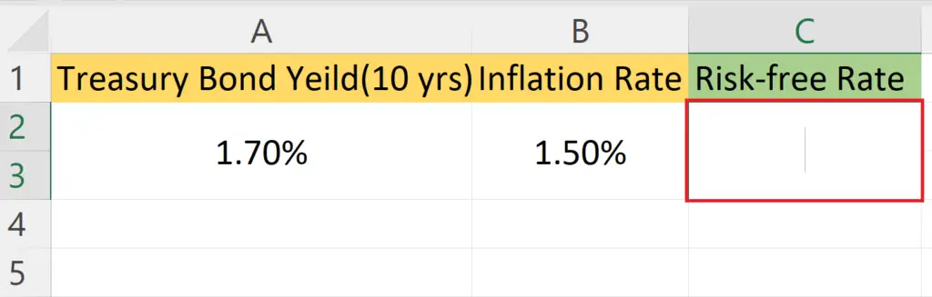
• Select a blank cell where you want to calculate the Risk-free rate using the treasury yield.

Step 2 – Place an Equals Sign

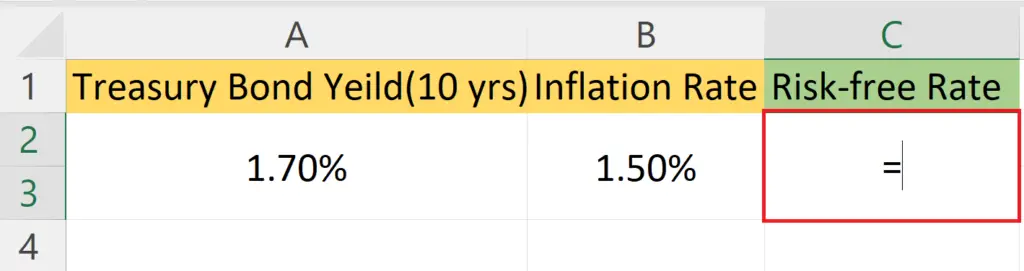
• Place an Equals sign in the blank cell.

Step 3 – Subtract the Inflation Rate from Treasury Yield

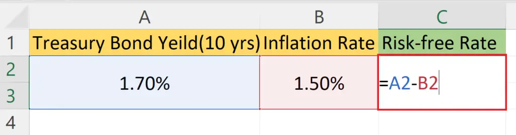
• Subtract the Inflation rate from the Treasury yield i.e. A2-B2.
• Where A2 and B2 are the cells containing the Treasury Yield Rate for 10 yrs and the Inflation rate, respectively.

Step 4 – Press the Enter Key

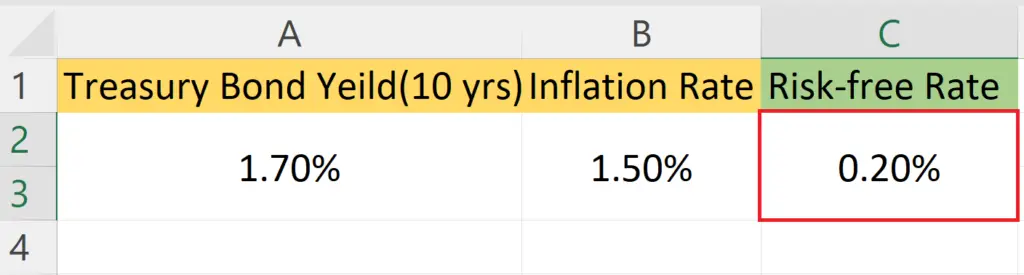
• Press the Enter key,
• The Risk-free rate using the Treasury Yield will be returned.

Method 2 – Historical Returns

Suppose you want to calculate the risk-free rate for a 10-year investment, but there is no Treasury security that matches your horizon. Instead, you decide to use historical returns on high-grade corporate bonds. You find that the average return over the past 10 years was 3.5%. 

You adjust this for inflation by subtracting the inflation rate to get the real risk-free rate.

Step 1 – Select a Blank Cell

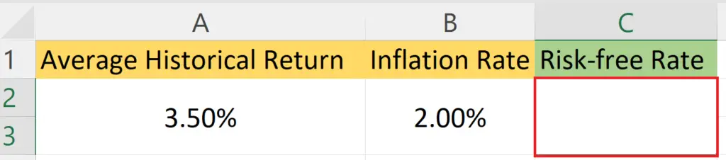
• Select a blank cell where you want to calculate the Risk-free rate using the Historical returns.

Step 2 – Place an Equals Sign

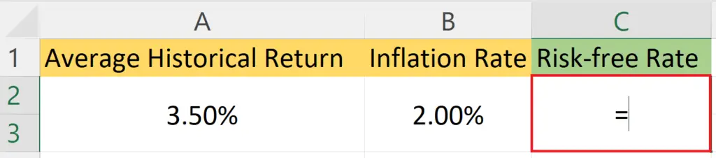
• Place an Equals sign in the blank cell.

Step 3 – Subtract the Inflation Rate from Average Historical Return

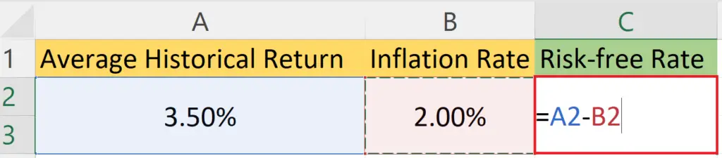
• Subtract the Inflation rate from the average Historical return i.e. A2-B2.
• Where A2 and B2 are the cells containing the historical return rate for 10 yrs and the Inflation rate, respectively.

Step 4 – Press the Enter Key

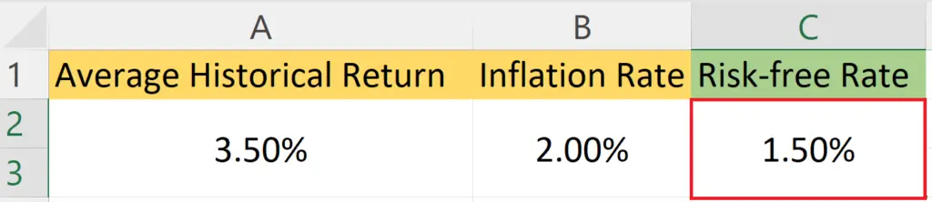
• Press the Enter key,
• The Risk-free rate using the Historical returns will be returned.

Method 3: Market Risk Premium

The market risk premium is the additional return an investor expects to receive over the risk-free rate to compensate for taking on the risk of investing in the stock market. Suppose you want to calculate the risk-free rate for a 10-year investment, and you believe that the expected return on the S&P 500 is 8%. You go to the Treasury Department’s website and find that the yield on a 10-year Treasury bond is 1.7%. You subtract the Treasury yield from the expected return on the S&P 500 to get the market risk premium. Then, you adjust the market risk premium for inflation to get the real risk-free rate.

Step 1 – Select a Blank Cell and Place an Equals Sign

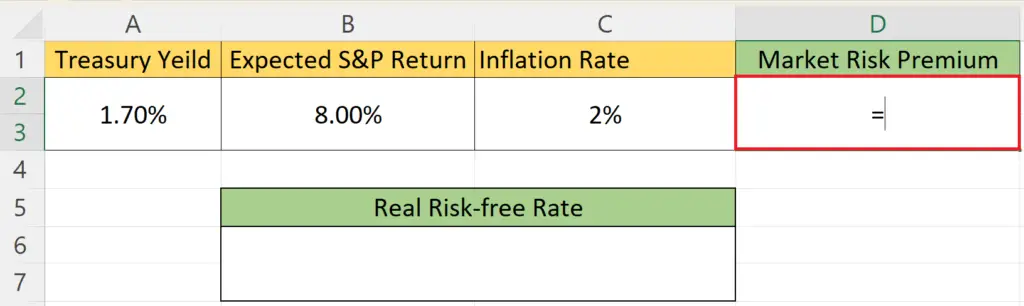
• Select a blank cell to calculate the Market Risk Premium.
• Place an Equals sign in the cell.

Step 2 – Subtract The Treasury Yield from the Expected S&P Return

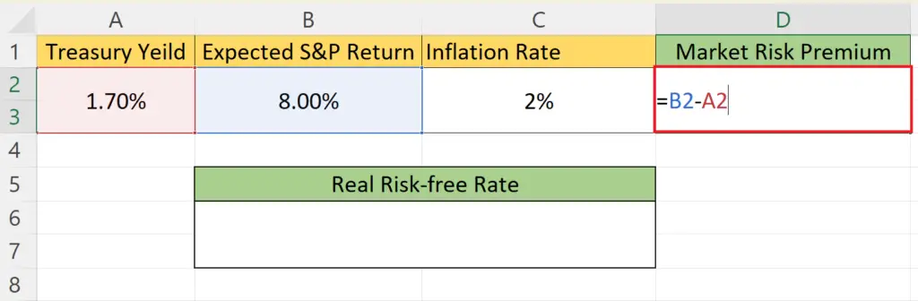
•  Subtract The Treasury Yield from the Expected S&P Return i.e. B2-A2.
• Where A2 is the cell containing the Treasury Yield and B2 is the cell containing the S&P return.

Step 3 – Press the Enter Key

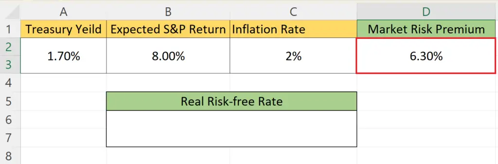
• Press the Enter key to calculate the Market Risk Premium.

Step 4 – Subtract the Inflation Rate from the Market Risk Premium

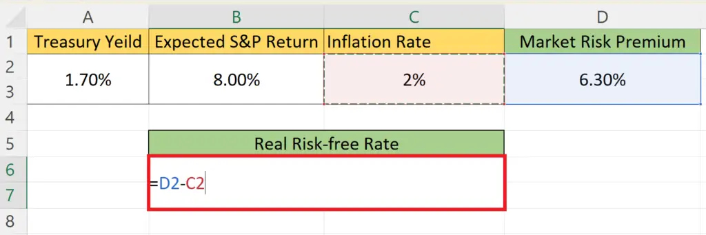
• Subtract the Inflation rate from the Market Risk Premium i.e. D2-C2.

Step 5 – Press the Enter Key

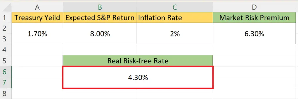
• Press the Enter key to get the Real Risk-free rate.