
How to calculate class rank percentage in Excel
 By
SpreadCheaters
By
SpreadCheaters
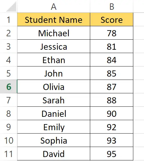
Here we have a dataset that contains Student Names and Scores. We will be calculating how to calculate the class rank percentage by following the simple steps below. Let’s have a look at the dataset first.
Calculating class rank percentages can provide valuable insights into student performance and help identify top performers within a class. Excel, with its powerful functions and formulas, offers a convenient way to calculate and analyze class rank percentages. In this blog post, we will guide you through the steps to calculate class rank percentages using Excel.
Step – 1 Find the rank of the students.
– We will type the following formula to find the rank of students.
– Rank finding formula :
=RANK(B2,$B$2:$B$11,0)
– Formula explanation:
“=RANK“: This is the function name. In this case, it represents the RANK function in Excel.
“B2“: This is the value for which you want to calculate the rank. In this example, it refers to the value in cell B2.
“$B$2:$B$11“: The following is the range of values for which you want to calculate the rank. In this example, it refers to the range from cell B2 to B11. The dollar signs ($) right before the column and row references make the range absolute, which means it won’t change when the formula is copied to other cells.
“0“: This is the optional argument that evaluates the ranking order. A value of 0 (zero) indicates descending order, where the highest value receives the rank of 1.
Step – 2 Find the rank for the rest of the students.
– Select the cell with the formula from the bottom right, when the ‘+’ sign appears.
– Click and drag it to the rest of the cells as shown above.
Step – 3 Finding the percentage of the rank.
– Now we will find the percentage for rank.
– The formula we used for finding the percentage of the rank is:
=C2/COUNT(B$2:B$11)
– Formula explanation:
“=C2“: This refers to the value you want to calculate the rank percentage for. In this example, it refers to the value in cell C2.
“/“: This is the division operator, used to divide the value by another.
“COUNT(B$2:B$11)“: This function counts the number of values in the range B$2:B$11. The dollar signs ($) before the column and row references make the range absolute, which means it won’t change when the formula is copied to other cells.
Step – 4 Calculate the rank percentage for the rest of the students.
– Select the cell with the formula from the bottom right, when the ‘+’ sign appears.
– Click and drag it to the rest of the cells as shown below.
– After that, in the Home tab go to the Number group and click on the ‘%’ sign.


