How to automatically number rows in Google Sheets

Google Sheets is a powerful tool for organizing and analyzing data. One common task when working with data is to number rows to make it easier to reference and manipulate the data. While you can manually number rows, this can be time-consuming and prone to errors. Fortunately, Google Sheets offers a few different ways to automatically number rows.

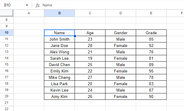
Here in this tutorial, we will learn how to automatically number rows in Google Sheets. We have a dataset on which we will automatically apply row numbers using two different methods by following the steps below. Let’s have a look at the dataset first. 

Method – 1 Row Formula

Step – 1 Type the Formula.

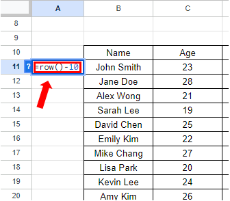
• Select the cell where you want to type the formula.
• Syntax of the formula is

=row() – Value   

Value: Row number from where your dataset starts. 

• In our case formula will be

=row() – 10 

Step – 2 Find values for the rest of the cells. 

• Select the cell that contains the formula.
• Drag that cell from the bottom right to the rest of the cells.
• All the remaining values will appear automatically.

Method – 2 Autofill the cells.

Step – 1 Select the first two row numbers.

• In the first-row type the first number.
• In the second-row type the second number.
• Select both cells.

Step – 2 Autofill the cells.

• After selecting the first two cells drag them from the bottom right of the cell to the rest of the cells.
• Values will appear automatically.

Conclusion:

These methods for automatically numbering rows in Google Sheets can save you time and reduce errors in your data. Depending on the size and complexity of your data, one method may be more suitable than the other. Try them out and see which one works best for your needs.