How to automatically alphabetize in Google Sheets

Automatically alphabetizing in Google Sheets means sorting a range of data in alphabetical order based on a chosen column, row, or a combination of columns or rows. This is an important sorting process that is used commonly in Spreadsheets. This feature is helpful for organizing data and making it easier to find specific entries in large data.

In this tutorial, we will learn how to automatically alphabetize in Google Sheets. Google Sheets offers three ways to automatically alphabetize data. The SORT function sorts data in alphabetical order based on a column or range, the FILTER function filters data in alphabetical order based on a column or range, and the “Data” menu can be used to sort or filter data in alphabetical order.

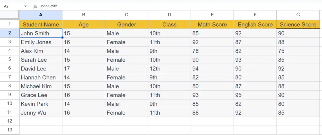
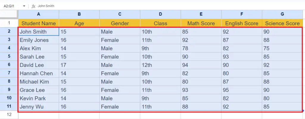
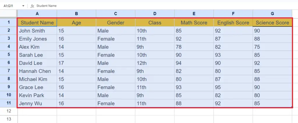
Currently, we have a data set representing the academic details of some students. We want to sort the data alphabetically on the basis of names i.e. the first column ( A ) so that it is easier to find the record of any student. 

Method 1: Using the SORT Function 

Step 1 – Select a Blank Cell and Place an Equals Sign

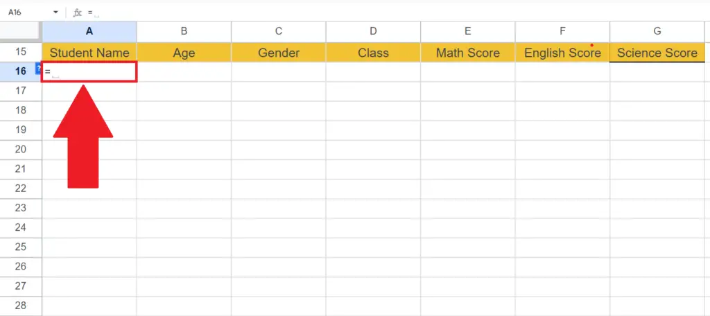
• Select a blank cell, where you want to print the alphabetized data.
• Place an Equals sign in the blank cell.

Step 2 – Enter the SORT Function

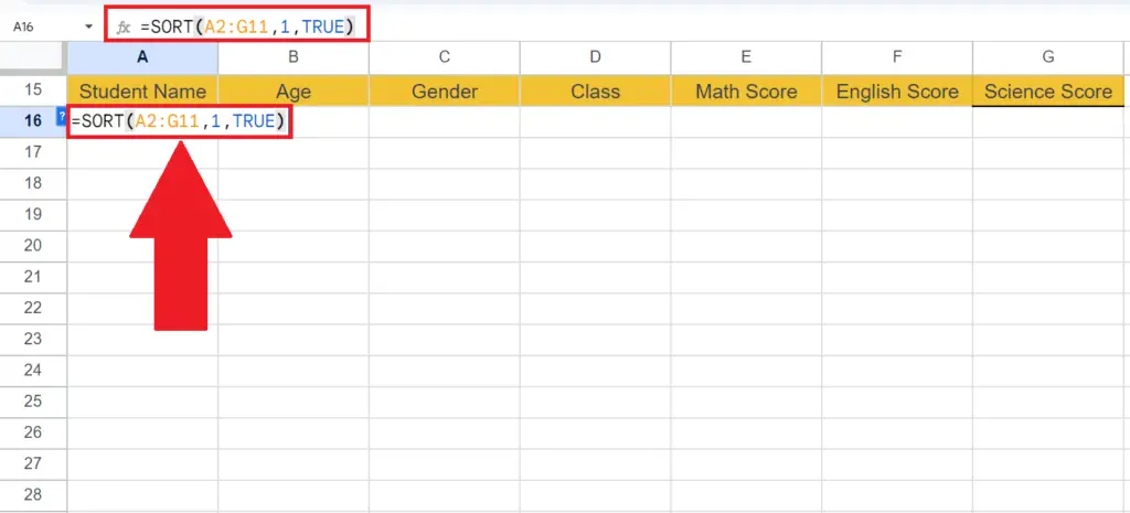
• The SORT function is a built-in function in Google Sheets.
• The syntax of the SORT function is:

                   SORT(A2:G11,1,TRUE)

The first argument is the range of the data to be sorted.

The second argument i.e. 1, represents the main column in the data on the basis of which sorting will be performed.

The third argument is the sorting type i.e “TRUE” for A to Z and  “False” for  Z to A.

Step 3 – Press the Enter Key

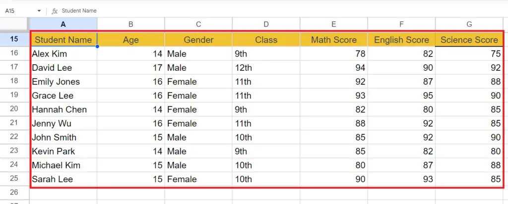
• Press the Enter key to automatically alphabetize the data.

Method 2: Using the built-in Sort option from Data Menu

Step 1 – Select the Data

• Select the Data to be sorted.

Step 2 – Click on the Data Menu

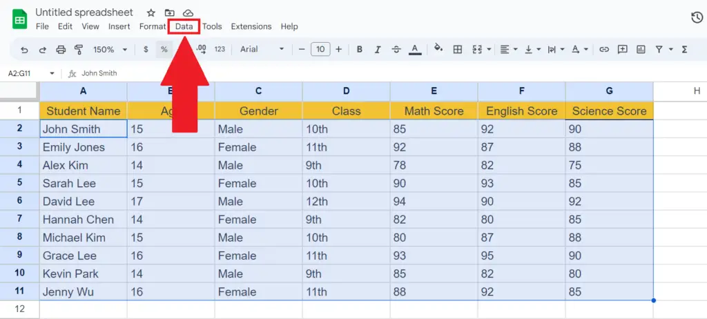
• Click on the Data menu in the menu bar.

Step 3 – Click on the “Sort range” Option

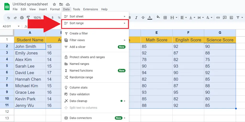
• Click on the “Sort range” option in the “Data” menu.

Step 4 – Click on the Sorting Type

• Click on the type of sorting required i.e. A-Z or Z-A.
• The data will be automatically alphabetized.

Method 3: Using Filter Feature

Step 1 – Select the Data

• Select the Data to be sorted.
• When using the Filter feature, we need to include the headers in the selection. 

Step 2 – Click on the Filter Button 

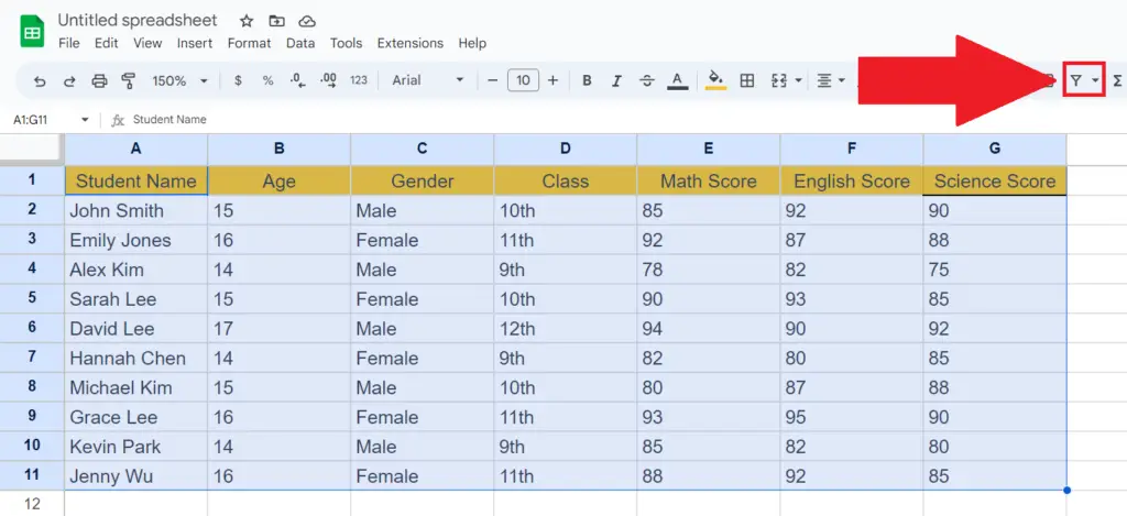
• Click on the Filter button in the ribbon.
• Filter drop-down arrows will appear next to each column header.

Step 3 – Click on the Filter Arrow

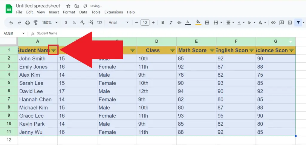
• Click on the filter arrow of the column on the basis of which sorting is to be done. 
• A drop-down list will appear.

Step 4 – Select the Sorting Type

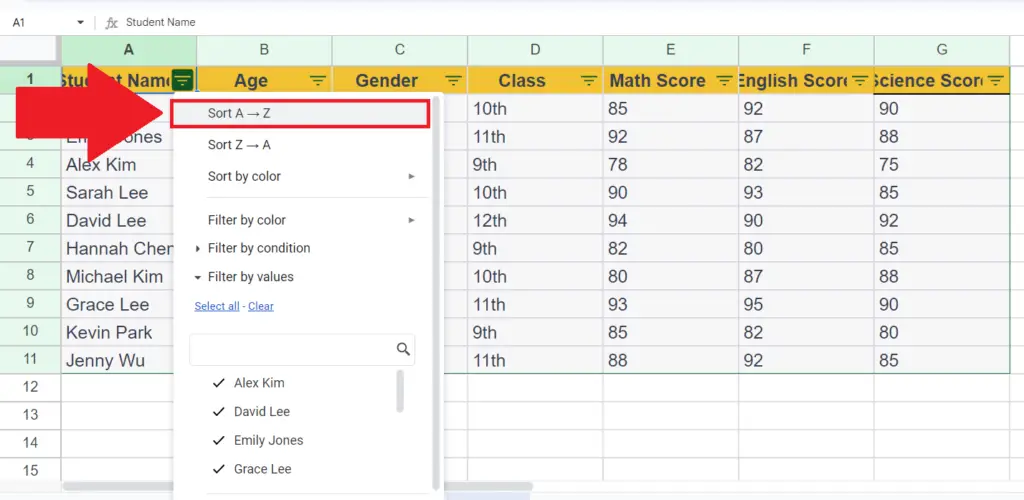
• Select the type of sorting required i.e. Sort A-Z or Sort Z-A, listed at the start of the list.
• The data will be automatically alphabetized.

Step 5 – Click on the Filter Arrow

• Click on the Filter arrow to disable the Filter arrows.