How to auto number in Google Sheets

Google Sheet is a powerful tool for managing data and information, but manually numbering rows or columns can be a tedious and time-consuming task. Fortunately, Google Sheets offers a simple solution with the “Auto Numbering” feature that automatically assigns numbers to rows or columns.

Here we have a dataset, in this dataset, there are Cars and their Quantity. Now we want to add a serial number to the column of Cars to make it easier to read. In this tutorial, we will autonumber in Google Sheets but first let’s take a look at the dataset.

Method – 1 Using Row Function.

Step – 1 Insert the column.

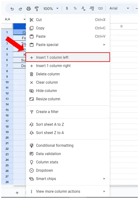
• Select the column that you want to number.
• Right-click and select the Insert 1 column left option.
• This will add a column on the left side.

Step – 2 Adding the Row function.

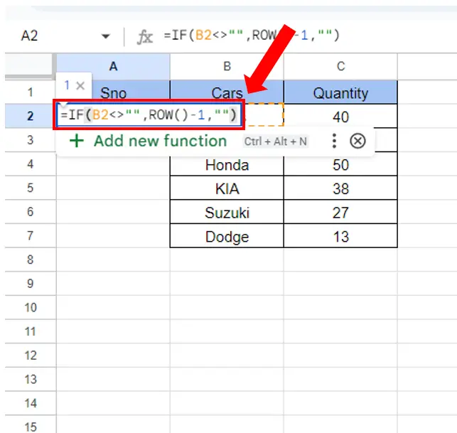
• In cell A2 add the ROW formula.
• Syntax of the formula will be

=IF(Cell_Address<>””,ROW()-1,””)

• In our case the formula will be

=IF(B2<>””,ROW()-1,””)

Step – 3 Numbering the rest of the cells.

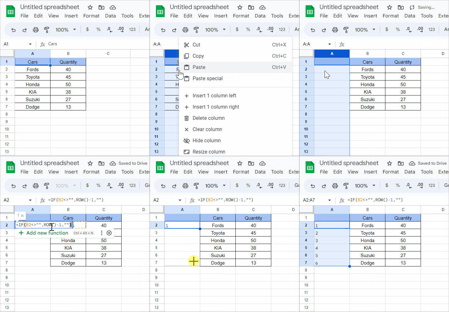
• Select the cell that contains formula.
• Drag from the bottom right to the rest of the cells.
• The cells will be numbered.

Method – 2 Using Fill Handle.

Step – 1 Insert the column.

• Select the column which you want to number.

• Right-click and select the Insert 1 column left option.
• This will add a column on the left side.

Step – 2 Number the cells.

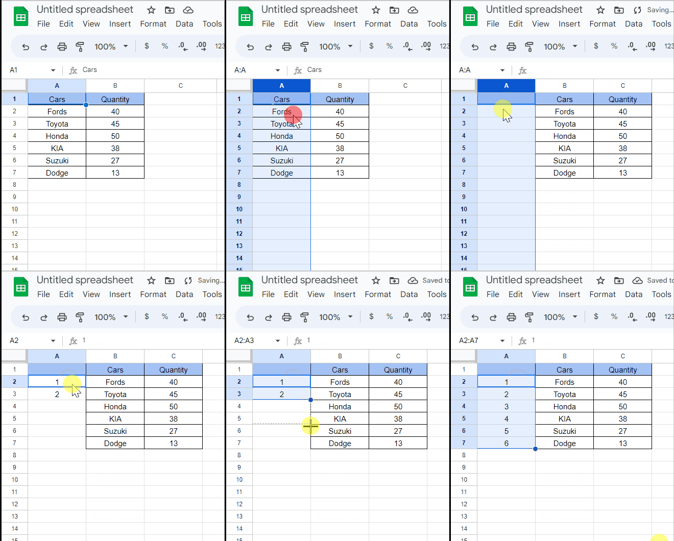
• Write 1 in cell A2 and 2 in cell A3.
• Then select cell A2 and A3.
• Use the Fill Handle tool to fill the rest of the cells.

Method – 3 Using SEQUENCE function.

Step – 1 Insert the column.

• Select the column you want to number.

• Right-click and select the Insert 1 column left option.
• This will create a column on the left side of the selected column.

Step – 2 Apply the formula.

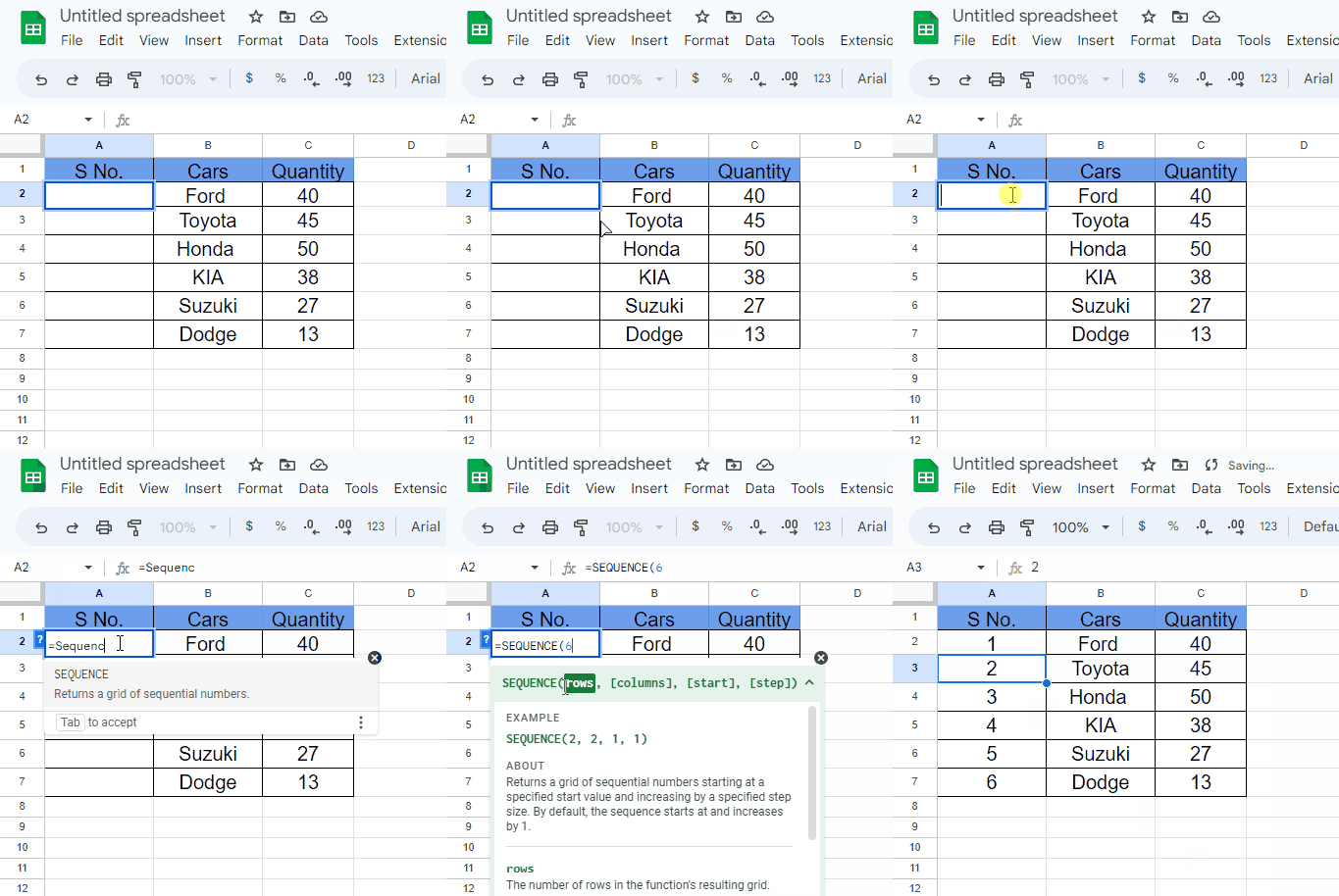
• Select the cell where you want to type the formula. In our case we selected cell A2.
• Syntax of the formula is

SEQUENCE(Row_Number)

• In our case formula will be

SEQUENCE(6)

We used 6 because we have 6 rows to number.