How to aggregate data in Google Sheets

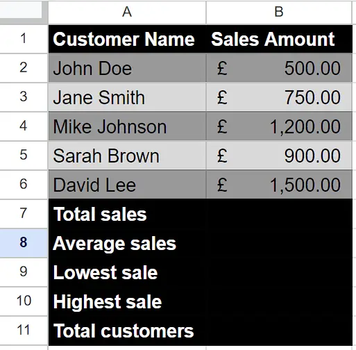
We have a dataset that includes customer names and sales information. To analyze and aggregate this data, we will explore how to utilize SUM, AVERAGE, COUNT, MAX, and MIN functions for aggregating the sales data.

Understanding Functions and their syntax

SUM Function:

The SUM function in Google Sheets is used to calculate the total sum of a range of values. It allows you to add up numbers and cell references within a specified range.

The syntax of the SUM function is as follows:

=SUM(value1, value2, …)

value1, value2, … –  These are the values or cell references you want to include in the sum. You can specify multiple values or ranges separated by commas.

AVERAGE Function:

The AVERAGE function in Google Sheets is used to calculate the arithmetic mean of a range of numbers. It calculates the sum of the numbers in the specified range and divides it by the count of those numbers.

The syntax of the AVERAGE function in Google Sheets is:

=AVERAGE(value1, value2, …)

value1, value2, and so on: These are the numerical values or ranges for which you want to calculate the average. You can specify up to 30 values or ranges as arguments.

Note that the AVERAGE function automatically ignores empty cells, cells containing text, and cells with logical values (such as TRUE or FALSE) in the range.

MIN Function:

In Google Sheets, the MIN function is used to find the smallest value in a range of cells or a list of values. It returns the minimum value from the specified range.

The syntax of the MIN function in Google Sheets is as follows:

=MIN(value1, value2, …)

value1, value2, and so on: These are the values or cell references that you want to compare to find the minimum value. You can provide multiple values as arguments separated by commas, or you can provide a range of cells as an argument.

MAX Function:

In Google Sheets, the MAX function is used to find the maximum value within a given range or a set of specified values. It returns the highest value in the dataset.

The syntax for the MAX function in Google Sheets is as follows:

=MAX(value1, [value2, …])

value1, value2, etc.: These are the values or cell references that you want to evaluate. You can provide multiple values as separate arguments, separated by commas.

You can also specify a range of cells using the colon (:) notation. For example, A1:A10 represents cells from A1 to A10.

COUNTA Function:

The COUNTA function is a popular function used in spreadsheet applications, such as Microsoft Excel or Google Sheets, to count the number of cells that contain any value (including numbers, text, or logical values like TRUE or FALSE) within a specified range.

The syntax of the COUNTA function is as follows:

=COUNTA(value1, value2, …)

value1, value2, and so on: These are the individual values or ranges that you want to count.

The COUNTA function takes one or more arguments, separated by commas. Each argument represents a range or a value that you want to include in the count. The function counts both empty cells and non-empty cells.

In Google Sheets, aggregation refers to the process of combining and summarizing data from multiple cells or ranges into a single value. It allows you to perform calculations on a set of data to derive meaningful insights or obtain a consolidated result. In Excel, there is a function called “AGGREGATE” that provides a wide range of aggregation options. It allows you to perform calculations on a data set while also offering the flexibility to choose specific functions such as SUM, AVERAGE, COUNTA, MAX, and MIN within a single formula. However, in Google Sheets, there isn’t an equivalent “AGGREGATE” function that combines all these functionalities into one. Instead, you can use the individual aggregation functions separately in Google Sheets to achieve similar results.

Step 1 – Use the “SUM” Function

– Select any empty cell where you wish to use the “SUM” function to sum values.
– Then, press = (equal sign) on your keyboard.
– After that, write SUM and choose SUM Function by using the tab button.
– Now, enter the cell range whose values you wish to sum up.
– For example, we wish to sum up values of range (B2:B6) then we will write the formula,

Step 2 – Use the “AVERAGE” Function

– Choose an empty cell where you want to display the average.
– Begin by typing the equal sign (=) on your keyboard.
– Follow the equal sign with the word “AVERAGE” and select the AVERAGE function using the tab button or by manually typing it.
– Specify the cell range for which you want to calculate the average.
– For instance, if you want to average values in the range B2 to B6, you would write the formula above,

Step 3 – Use the “MIN” Function

– Select an empty cell where you want to show the lowest value.
– Start by typing the equal sign (=).
– After the equal sign, enter the word “MIN” and select the MIN function either by using the tab button or by manually typing it.
– Select the cell range for which you want to determine the lowest value.
For example, if you want to find the lowest value in the range B2 to B6 then, write this formula

Step 4 – Use the “MAX” Function

– Choose an empty cell where you want to display the highest value.
– Begin by typing the equal sign (=).
– After the equal sign, enter the word “MAX” and select the MAX function either by using the tab button or by manually typing it.
– Specify the cell range for which you want to determine the highest value.
For instance, if you want to find the highest value in the range B2 to B6 then, type this formula

Step 5 – Use the “COUNTA” Function

– Choose an empty cell where you want to display the total customers.
– Begin by typing the equal sign (=).
– After the equal sign, enter the word “COUNTA” and select the COUNTA function either by using the tab button or by manually typing it.
– Specify the cell range in which the name of each customer is entered.
– For instance, we have selected the range B2 to B6 and written the formula,