How to add a range in Google Sheets

In Google Sheets, a range refers to a group of cells within a spreadsheet that is selected together. Adding a range allows you to perform various tasks, such as applying a formula or function to a specific set of cells, formatting a range of cells, or creating a chart based on the data in the range.

In this tutorial, we will learn how to add a range in Google Sheets. Adding a range of cells in Google Sheets is straightforward and can be accomplished using the SUM function. To reference a range, one can use a colon (:) or click and drag the mouse to select a contiguous range. However, for a non-contiguous range, one must select the range by holding the CTRL key or adding the reference of each cell, separated by a comma.

Method 1: Adding a Contiguous Range Using a Colon

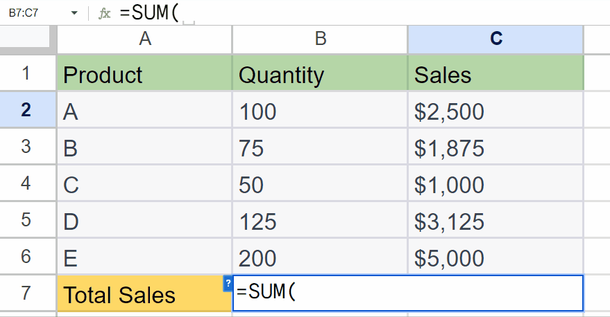
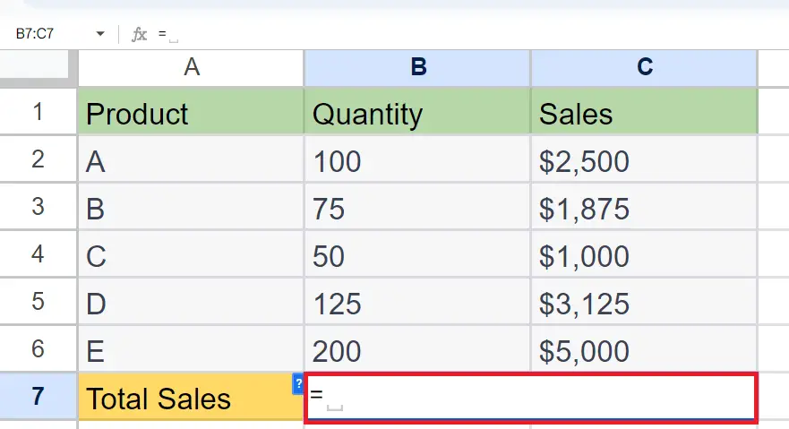
Step 1 – Select a Blank Cell and Place an Equals Sign

• Select a blank cell.
•  Place an Equals sign in the blank cell.

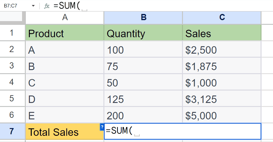
Step 2 – Enter the SUM Function 

• Enter the SUM function next to the Equals sign.
• Open the parentheses.

Step 3 – Enter the Reference of the First Cell

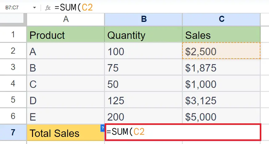
• Enter the reference of the first cell of the range to be added.

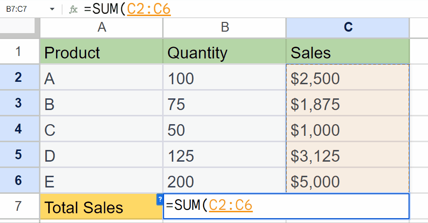
Step 4 – Place a Colon

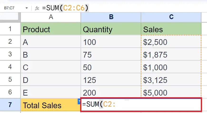
• Place a colon ( : ) next to the reference of the first cell.

Step 5 – Enter the Reference of the Last Cell

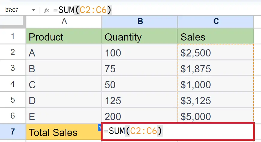
• Enter the reference of the last cell of the range to be added.
• Close the parentheses.

Step 6 – Press the Enter Key

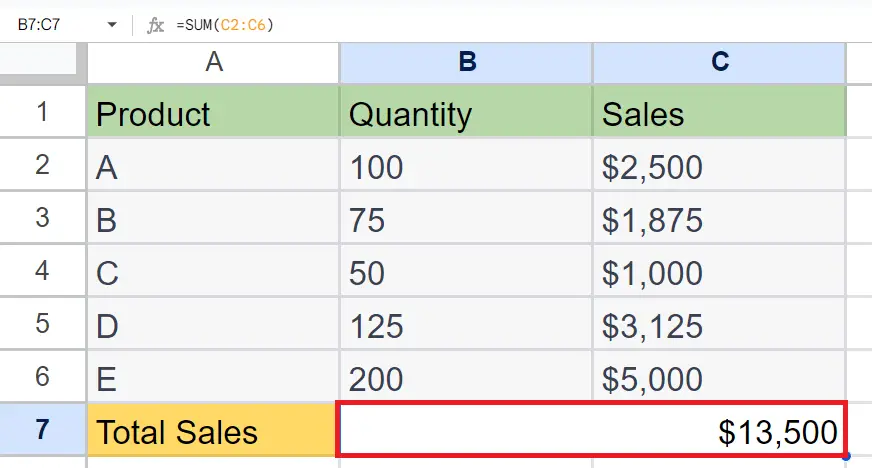
• Press the Enter key to add the range.

Method 2: Using the Cursor to Add the Range

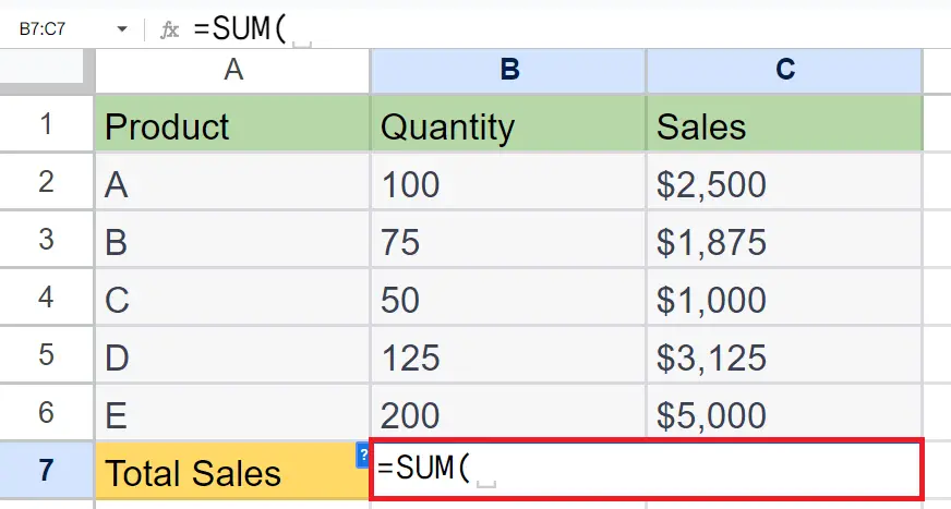
Step 1 – Select a Blank Cell and Place an Equals Sign

• Select a blank cell.
•  Place an Equals sign in the blank cell.

Step 2 – Enter the SUM Function 

• Enter the SUM function next to the Equals sign.
• Open the parentheses.

Step 3 – Hover the Cursor over the First Cell

• Hover the cursor over the first cell of the range.

Step 4 – Select, Drag, and Drop the Cursor

• Select the first cell.
• Drag the cursor over the range of cells you want to add.
• Drop the cursor on the last cell.

Step 5 – Close the Parenthesis and Press the Enter Key

• Close the parenthesis of the SUM function.
• Press the Enter key.
• The contiguous range will be added.

Method 3: Adding a Non-Contiguous Range Using the CTRL Key

Step 1 – Select a Blank Cell and Place an Equals Sign

• Select a blank cell.
•  Place an Equals sign in the blank cell.

Step 2 – Enter the SUM Function 

• Enter the SUM function next to the Equals sign.
• Open the parentheses.

Step 3 – Press and Hold the CTRL Key and Select the Cells

• Press and Hold the CTRL key.
• Select the cells of the non-contiguous range individually.

Step 4 –  Close the Parenthesis and Press the Enter Key

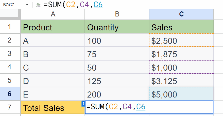
• Close the parenthesis of the SUM function.
• Press the Enter key.
• The non-contiguous range will be added.

Method 4: Adding a Non-Contiguous Range Manually

Step 1 – Select a Blank Cell and Place an Equals Sign

• Select a blank cell.
•  Place an Equals sign in the blank cell.

Step 2 – Enter the SUM Function 

• Enter the SUM function next to the Equals sign.
• Open the parentheses.

Step 3 – Enter the Reference of Each Cell and Separate Them Using a Comma

• Enter the reference of each cell and separate them using a comma i.e. B2, B4, B6.

Step 4 –  Close the Parenthesis and Press the Enter Key

• Close the parenthesis of the SUM function.
• Press the Enter key.
• The non-contiguous range will be added.