How do you get a cell in Excel to change color when a date expires? 

Conditional formatting in Excel is a useful method that allows you to change the color of cells based on specific conditions, such as when a date expires. This approach provides visual cues that quickly highlight expired dates, making it easier to identify and analyze time-sensitive information. By using conditional formatting, you can efficiently focus on relevant data and enhance the readability of your Excel spreadsheets. 

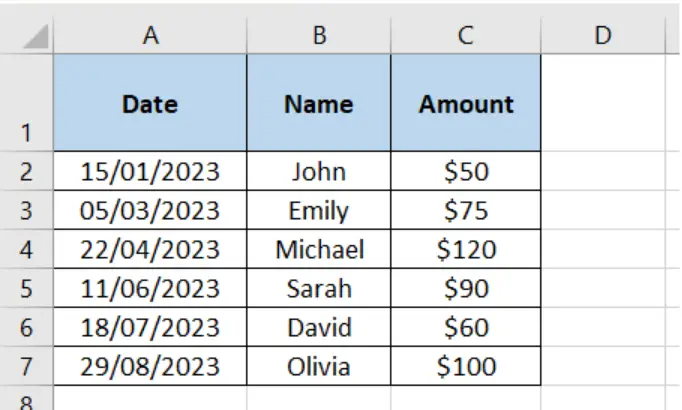
The provided data set includes Dates, Names, and corresponding Amounts. It represents a small sample of information where each row represents an entry with a specific date, person’s name, and an associated amount. The data set can be used for various purposes, such as tracking expenses, analyzing trends over time, or performing calculations and comparisons based on the given information. 

Step – 1  Go to New Rule from Conditional Formatting  

• Select the cell or range of cells to format. 
• Go to the “Home” tab in the Excel ribbon. 
• Click on the “Conditional Formatting” button. 
• Choose “New Rule” from the drop-down menu. 

Step – 2 Type the Formula   

• Click on the “New Formatting Rule” dialog box 
•  Select “Use a formula to determine which cells to format.” 
• Enter the formula that checks if the date in the cell has expired. For example, if your date is in cell A2, you can use the formula =A2<TODAY (). 

Step – 3 Change the format settings  

• Click on the “Format” button to choose the formatting options, including the desired background color. 
• After selecting the formatting options, click “OK” to close the dialog boxes. 

Formula explanation :  

The formula =A2<TODAY() compares the value in cell A2 with the current date. If the value in A2 is earlier than today’s date, the formula returns “TRUE“; otherwise, it returns “FALSE“. This formula is commonly used in conditional formatting to highlight cells when the associated date has already passed. 

Bonus Tip: 

Here are a few other conditions that you can use with the formula =A2<TODAY() in conditional formatting: 

Highlight dates of today or in the future: 

Formula: =A2>=TODAY() 

This condition will highlight dates in cell A2 or later, including today’s date. 

Highlight dates within a specific number of days from today: 

Formula: =AND(A2>=TODAY(), A2<TODAY()+7) 

This condition will highlight dates in cell A2 that are within the next 7 days (including today). 

Highlight dates older than a certain number of days from today: 

Formula: =A2<TODAY()-30 

This condition will highlight dates in cell A2 that are older than 30 days from today. 

Highlight past due dates with a custom number of days: 

Formula: =A2<TODAY()-15 

This condition will highlight dates in cell A2 that are more than 15 days past today’s date. 

You can adjust the formulas based on your specific requirements, such as changing the number of days or the comparison operator, to suit different date-based conditions in your conditional formatting.