
How to use conditional formatting to highlight values based on another cell
 By
SpreadCheaters
By
SpreadCheaters
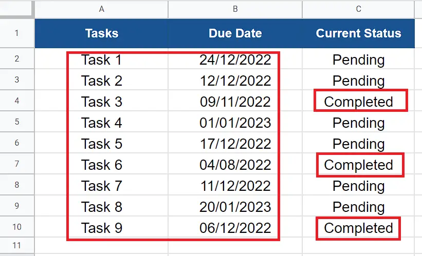
In this tutorial we will learn how to use conditional formatting to highlight cells based on the contents of other cells in Google Sheets. Let’s look at the dataset above, it has some tasks with due dates and their current status. We would like to highlight the tasks in the tasks column and their dates that have been marked as completed in the status column. So, we will highlight the data in column A and B based on the values in column C.
Let’s follow these simple steps to make it happen.

Conditional formatting in Google Sheets is a feature that allows you to apply formatting to cells in your spreadsheet based on certain conditions. This can be useful for highlighting important information or making your data easier to read and understand. For example, you could use conditional formatting to highlight cells based on the contents of other cells, cells that contain values that are above or below a certain threshold. This can help you quickly identify trends or patterns in your data and make your spreadsheet more visually appealing.
Step 1 – Select the data range that you wish to highlight
– First, we’ll select all the data that we wish to highlight, because this will decide the range to which we want to apply the conditional formatting.
Step 2 – Locate Conditional Formatting option
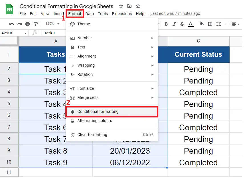
– Click on the Format tab in the list of main tabs.
– From the new dropdown menu, click on the Conditional formatting option as shown above.
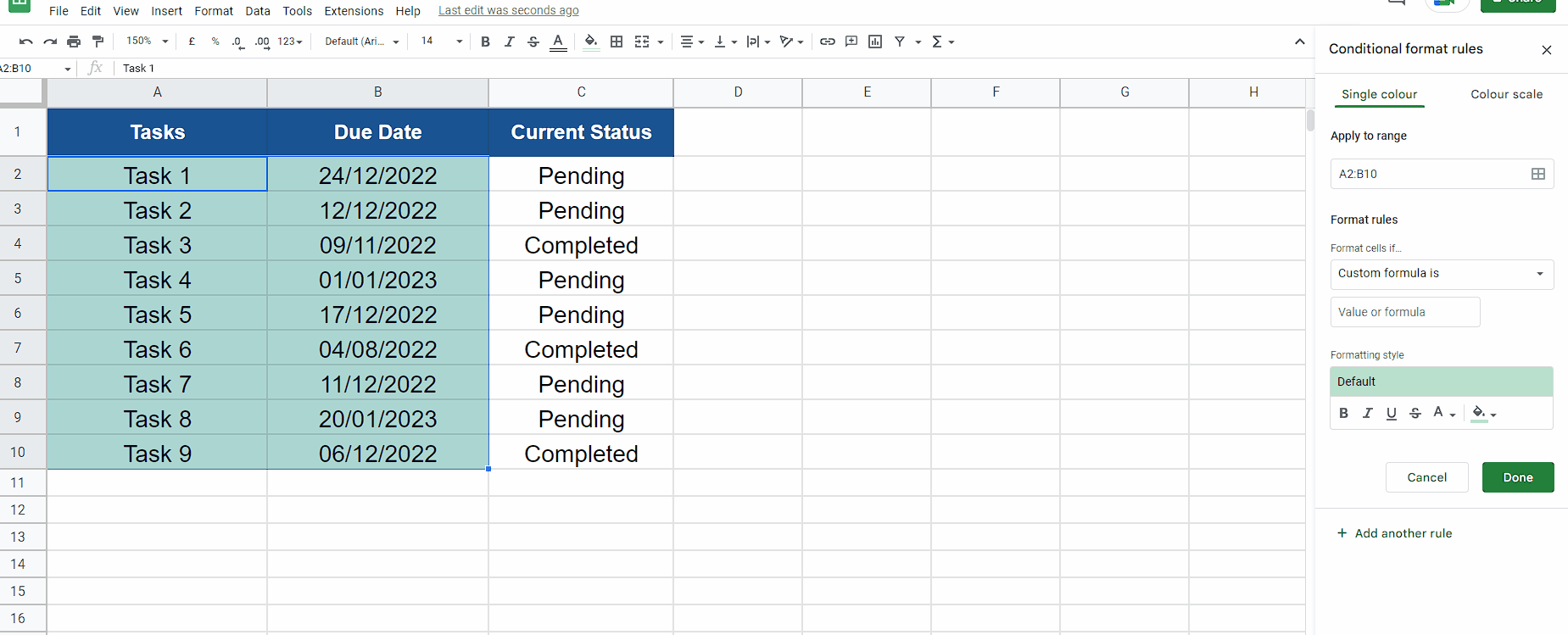
Step 3 – Use Custom Formula option in conditional formatting
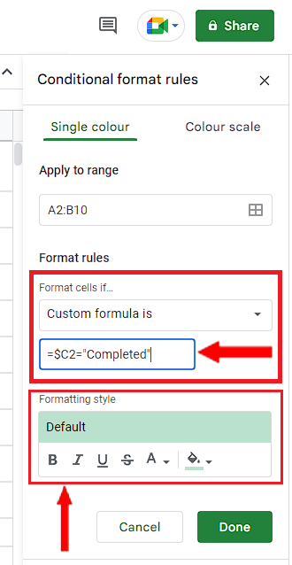
– The last action of the last step will open a sidebar in Google Sheets on the right side.
– In the Formal Rules options select the Custom Formula option and enter the following formula
=$C2=”Completed”
– Choose any color, font or other things from Formatting style or you can leave it to default as done in this example.
Step 4 – Implement the conditional formatting styles on the data
– After choosing your desired colors, fonts and other formatting styles. Press the Done button and it will apply the conditional formatting to the selected data range as shown above.


