
Filter by list in Microsoft Excel
 By
SpreadCheaters
By
SpreadCheaters
n this tutorial, we will learn how we can filter by list in Microsoft Excel. Filtering data by list is a useful task that is employed to extract specific data from a large data set. Mainly the FILTER function is utilized to perform this task.
The FILTER function in Excel allows you to extract data from a range based on specific criteria or conditions. It returns an array of values that meet the specified criteria, satisfying the filter conditions. The syntax of the FILTER function in Excel is as follows:
FILTER(array, include, [if_empty])
- array: This is the range or array of data that you want to filter.
- include: This is the criteria or condition that determines which values to include in the filtered result. It can be a range, an array, or a single value.
- [if_empty]: This is an optional parameter that specifies the value to return if the filtered result is empty. If omitted, it will return an empty array.
Let’s take an example to demonstrate how we can filter by list utilizing the FILTER function.
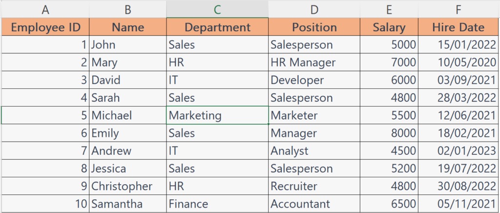
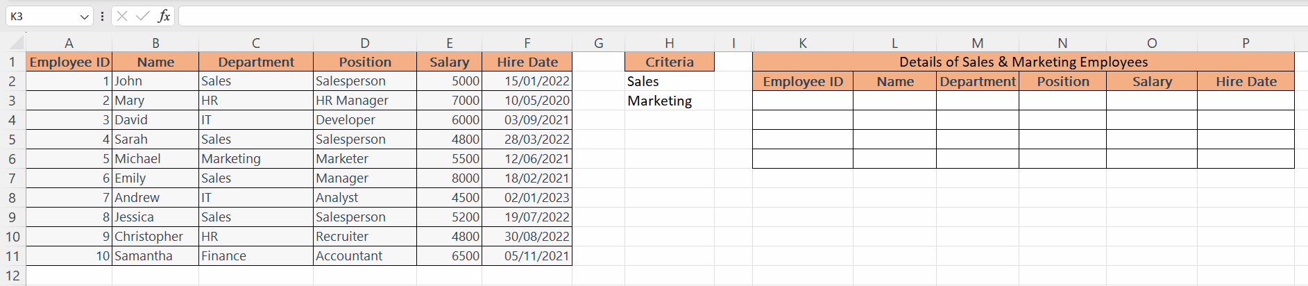
Right now, we have a data set that represents the employee details of a firm. We want to extract the details of employees of the “Sales” and “Marketing” departments only.
In Microsoft Excel, the “Filter by List” feature enables you to selectively filter data by specifying a particular list of values. This functionality proves advantageous when you wish to exhibit solely the rows that include specific values from a predefined list while concealing the rows that don’t correspond to those values.
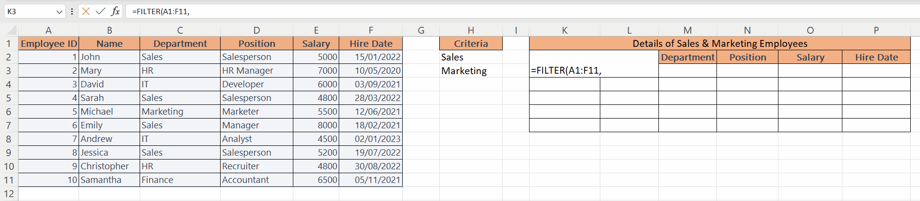
Step 1 – List the Criteria
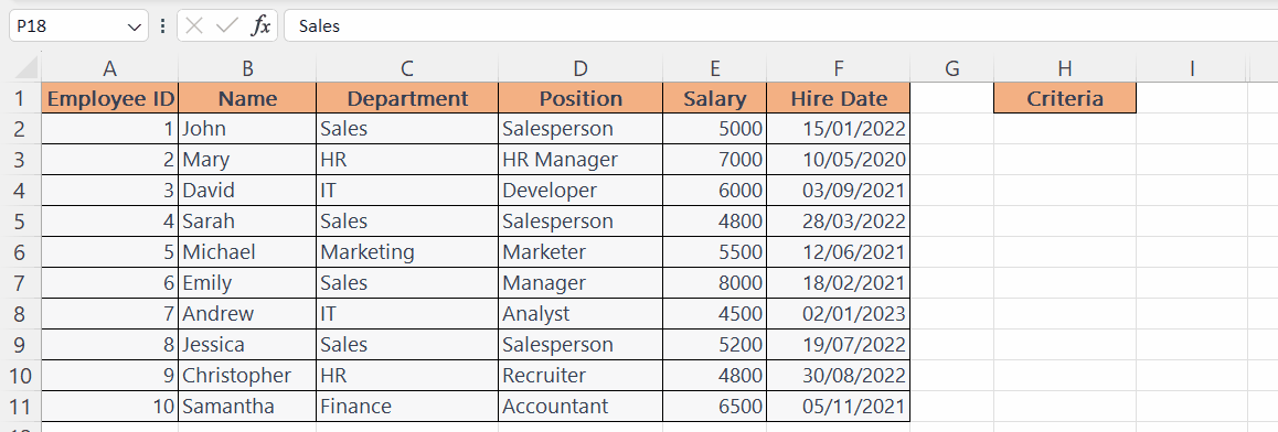
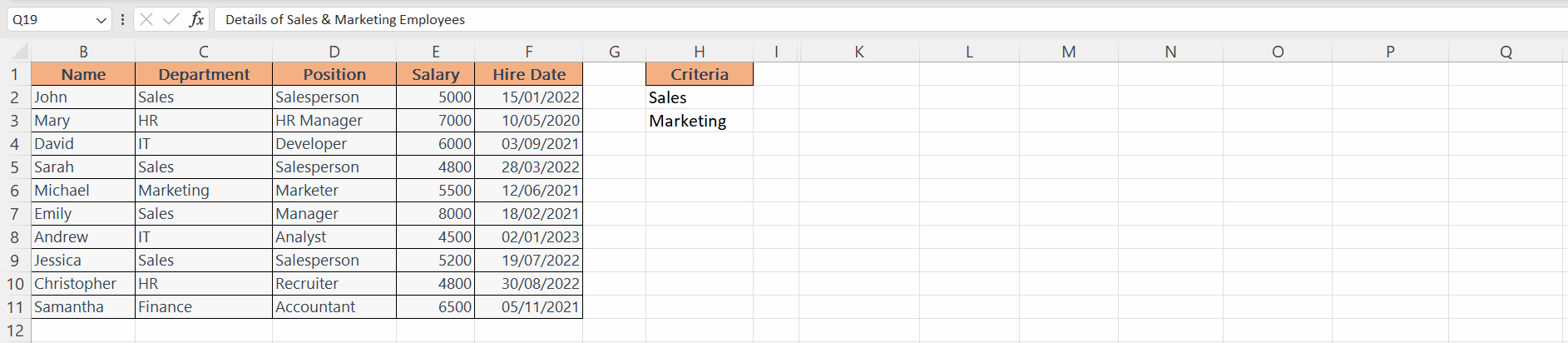
– In a separate column, list the values i.e. the criteria on the basis of which we aim to filter the values.
– Please note that the FILTER function in Excel operates in a “Case Sensitive” manner, meaning that the criteria you provide must match exactly.
Step 2 – Prepare the Headers
– Prepare the headers for the values i.e. copy the headers of the parent array and paste them on the destination.
– For this, we can utilize CTRL+C and CTRL+V shortcuts.
Step 3 – Enter the FILTER Function
– Enter the FILTER function in a blank cell, where the details would be displayed.
Step 4 – Input the “Array”
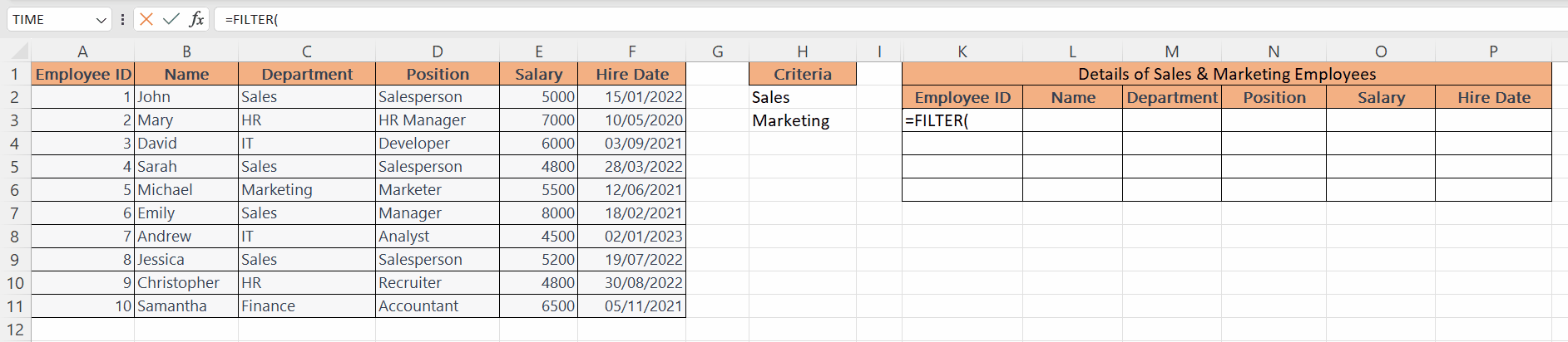
– Input the reference of the “Array” containing the details of employees.
FILTER(A1:F11,
Step 5 – Input the “Include” Parameter
– To specify the “Include” parameter, we will utilize the COUNTIF function.
– The structure of the function will be:
COUNTIF(H2:H3,C1:C11)
– The range “H2:H3” contains the criteria on the basis of which the data is to be extracted.
“C1:C11” is the column in the array, containing the criteria.
– The complete formula will be:
FILTER(A1:F11,COUNTIF(H2:H3,C1:C11))


