DATEDIF function in Google Sheets

The “DATEDIF” function in Google Sheets is a built-in formula used to determine the duration between two dates in terms of years, months, or days. The word “DATEDIF” is an abbreviation for “date difference.”

In this tutorial, we will learn how to utilize the DATEDIF function in Google Sheets. There are various methods by which we can use the DATEDIF functions. 

DATEDIF(start_date, end_date, unit)

start_date is the initial date or the earlier date.

end_date is the final date or the later date.

unit specifies the unit of measurement for the difference. 

Let’s say we have starting and ending dates for some projects. We aim to calculate the tenure of all the projects.

Method 1: Utilizing the DATEDIF Function to Calculate Tenure in Years Only

The DATEDIF function can be used to extract the number of years between two dates. We need to note that with DATED if we can only calculate complete years.

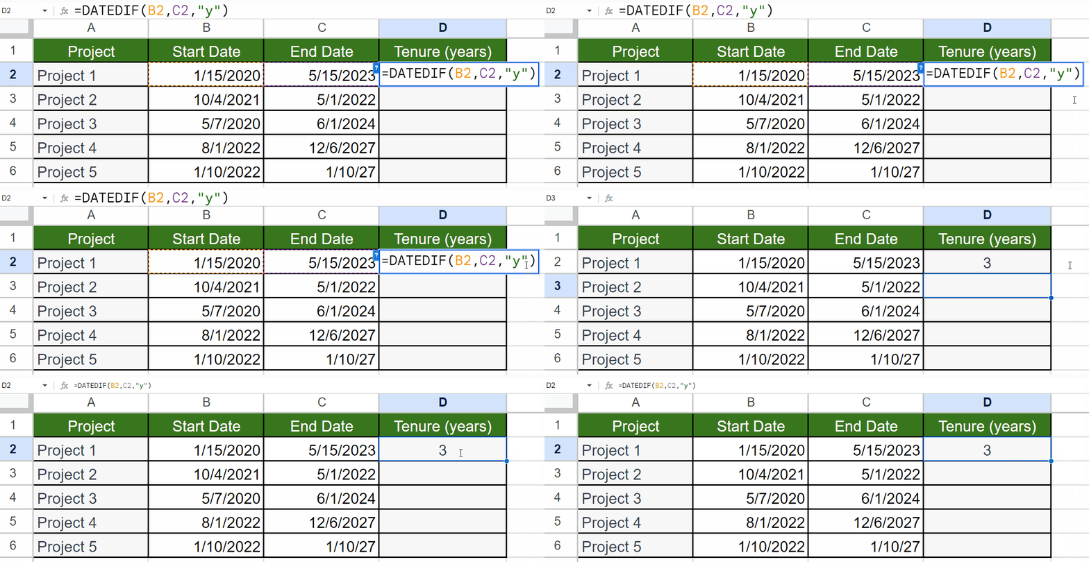
Step 1 – Utilize the DATEDIF Function

• Utilize the DATED function.
• The structure of the function would be:

DATEDIF(B2,C2,”Y”)

• The third parameter “Y” tells the function to extract years.

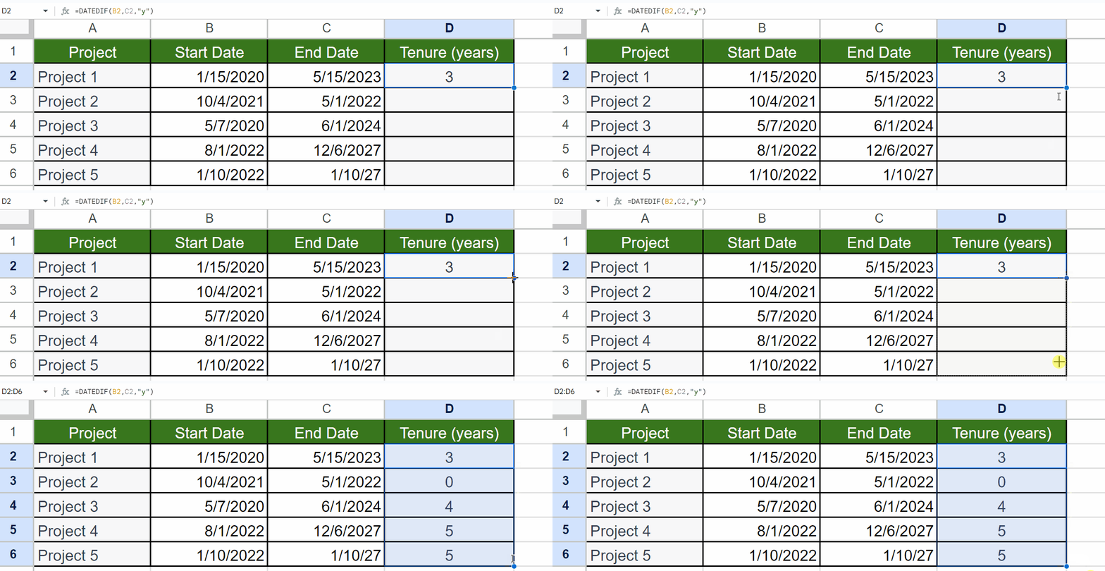
Step 2: Utilize Autofill to Calculate Years for Each Project

• With Autofill, we can apply the function to each project.

Method 2: Utilizing the DATEDIF Function to Calculate Tenure in Months Only

Certainly! You can use the DATEDIF function in Google Sheets to extract the number of months between two dates. By specifying the “M” or “m” unit in the DATEDIF formula, you can calculate the difference in complete months.

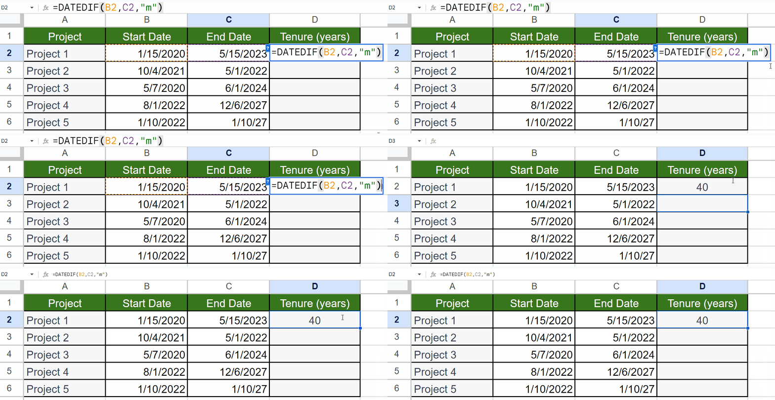
Step 1 – Utilize the DATEDIF Function

• Utilize the DATED function.
• The structure of the function would be:

DATEDIF(B2,C2, “m”)

• The third parameter “m” tells the function to extract months.

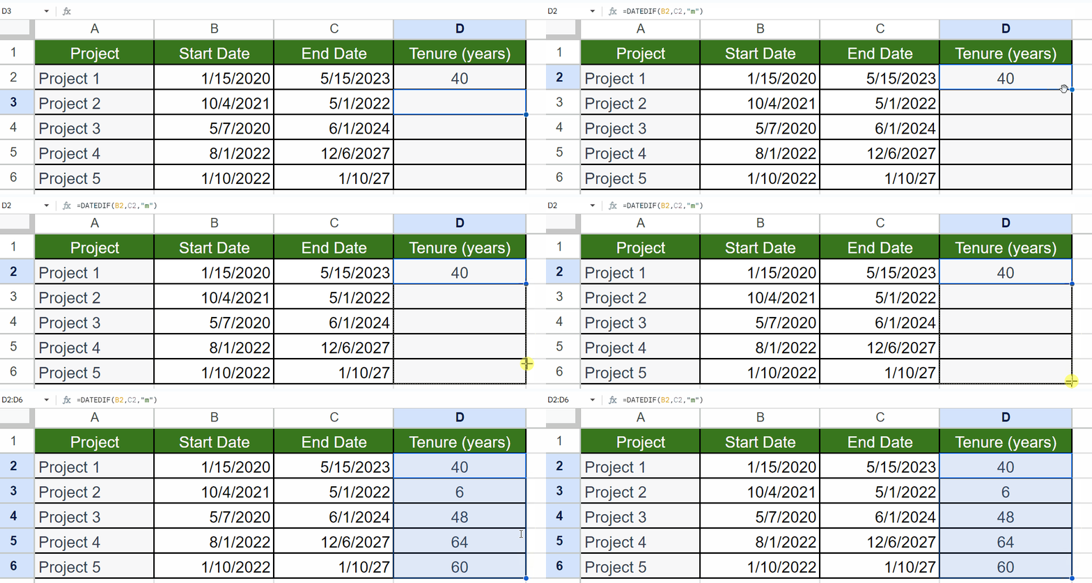
Step 2: Utilize Autofill to Calculate Years for Each Project

• With Autofill, we can apply the function to each project.

Method 3: Combining multiple DATEDIF Functions to Calculate Tenure in Years and Months

We can use two DATEDIF functions to calculate tenure in the “N years X months” format.

Step 1 – Input the First DATEDIF Function and Concatenating “Years” 

• Input the first DATEDIF function to extract years.

DATEDIF(B2,C2, “y”)

• Concatenate “years”:

            DATEDIF(B2,C2, “y”) & “ Years ”

Step 2 – Utilize DATEDIF to Extract the Remaining Months

• Write the following formula to concatenate “months” with the previous formula.

=DATEDIF(B2,C2, “y”) & ” Years “ & ((DATEDIF(B2,C2,“m”)-((DATEDIF(B2,C2,“y”)*12)) & ” Months”))

Here we have used the third DATEDIF to calculate complete years and multiplied it by 12. Then, we subtracted the result from the number of complete months calculated by the second DATEDIF function. This will give us the tenure in the required format.

Step 3 – Utilize Autofill to Calculate Tenure for Each Project

• Utilize Autofill to calculate tenure for each project.